Note
Go to the end to download the full example code.
Natural Earth map layers: lakes, rivers, glaciers, places#
esd.boundaries.natural_earth.load(aoi, layer=...) reads any of Natural
Earth’s public-domain vector layers by name, at 1:10m, 1:50m or 1:110m: lakes,
rivers and lake centrelines, coastline, land and ocean, glaciated areas,
populated places, boundary lines, and the point-of-view editions of the
countries layer. Each is one zipped shapefile, fetched once into the cache.
These layers are generalized for maps at their scale. They are the labels and outlines around snow data, not an analysis input: the glaciated areas here are a cartographic simplification of what the RGI glacier example measures.
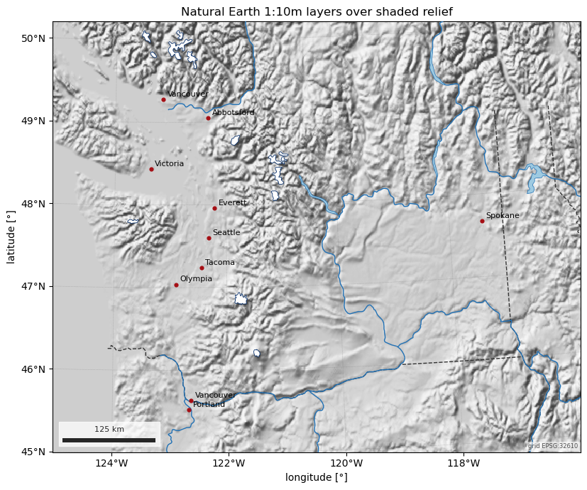
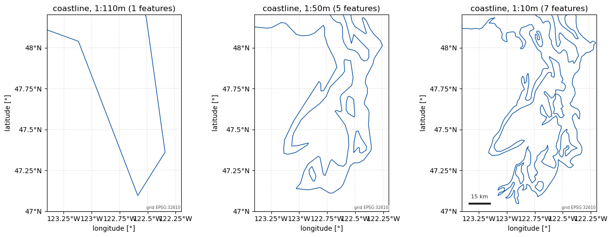
The figures build a context map of the Pacific Northwest over the Natural Earth hillshade, and compare the coastline of Puget Sound at the three scales.
import matplotlib.pyplot as plt

import easysnowdata as esd

aoi = (-125.0, 45.0, -116.0, 50.0)  # Puget Sound, the Cascades and the Columbia

box = esd.parse_aoi(aoi)
grid = box.to_geobox(crs="utm", resolution=1000)
print(box)
AOI(bounds=(-125.0000, 45.0000, -116.0000, 50.0000), clip=True)
The layers LAYERS knows, with
their category and scales; anything else in Natural Earth’s catalogue works
with category=.
admin_0_countries                    cultural  10m, 50m, 110m
admin_0_boundary_lines_land          cultural  10m, 50m, 110m
admin_1_states_provinces             cultural  10m, 50m
admin_1_states_provinces_lines       cultural  10m, 50m, 110m
populated_places_simple              cultural  10m, 50m, 110m
urban_areas                          cultural  10m, 50m
roads                                cultural  10m
coastline                            physical  10m, 50m, 110m
land                                 physical  10m, 50m, 110m
ocean                                physical  10m, 50m, 110m
lakes                                physical  10m, 50m, 110m
rivers_lake_centerlines              physical  10m, 50m, 110m
glaciated_areas                      physical  10m, 50m, 110m
antarctic_ice_shelves_polys          physical  10m, 50m
geography_regions_polys              physical  10m, 50m, 110m
geography_regions_elevation_points   physical  10m, 50m, 110m
Lakes, rivers, glaciated areas and populated places at 1:10m. Features are returned whole where they cross the AOI edge.
lakes_gdf = esd.boundaries.natural_earth.load(aoi, layer="lakes")
rivers_gdf = esd.boundaries.natural_earth.load(aoi, layer="rivers_lake_centerlines")
ice_gdf = esd.boundaries.natural_earth.load(aoi, layer="glaciated_areas")
places_gdf = esd.boundaries.natural_earth.load(aoi, layer="populated_places_simple")
borders_gdf = esd.boundaries.natural_earth.load(
    aoi, layer="admin_1_states_provinces_lines"
)
for label, frame_gdf in (
    ("lakes", lakes_gdf),
    ("rivers", rivers_gdf),
    ("glaciated areas", ice_gdf),
    ("places", places_gdf),
    ("state lines", borders_gdf),
):
    print(f"{label:16} {len(frame_gdf):4d} features")

cities_gdf = places_gdf[places_gdf["pop_max"] > 150_000].to_crs(grid.crs)
print(
    cities_gdf[["name", "pop_max"]]
    .sort_values("pop_max", ascending=False)
    .to_string(index=False)
)

hillshade_da = esd.terrain.hillshade.load(box.buffer(80_000), style="shaded-relief")
ax = esd.plotting.map(
    hillshade_da.odc.reproject(grid, resampling="bilinear"),
    cmap="gray",
    vmin=0,
    vmax=255,
    colorbar=False,
    title="Natural Earth 1:10m layers over shaded relief",
    figsize=(10, 7),
)
esd.plotting.add_outline(
    ax, borders_gdf, edgecolor="0.2", linewidth=1.0, linestyle="--"
)
esd.plotting.add_outline(ax, rivers_gdf, edgecolor="#2171b5", linewidth=1.0)
esd.plotting.add_outline(
    ax, lakes_gdf, facecolor="#9ecae1", edgecolor="#2171b5", linewidth=0.5
)
esd.plotting.add_outline(
    ax, ice_gdf, facecolor="white", edgecolor="#08306b", linewidth=0.6
)
ax.scatter(
    cities_gdf.geometry.x, cities_gdf.geometry.y, s=12, color="#a50f15", zorder=5
)
for _, city in cities_gdf.iterrows():
    ax.annotate(
        city["name"],
        (city.geometry.x, city.geometry.y),
        xytext=(4, 3),
        textcoords="offset points",
        fontsize=8,
        zorder=5,
    )
ax.figure.tight_layout()
  0%|                                              | 0.00/2.35M [00:00<?, ?B/s]
  0%|                                              | 0.00/2.35M [00:00<?, ?B/s]
100%|█████████████████████████████████████| 2.35M/2.35M [00:00<00:00, 14.8GB/s]

  0%|                                              | 0.00/2.08M [00:00<?, ?B/s]
  0%|                                              | 0.00/2.08M [00:00<?, ?B/s]
100%|█████████████████████████████████████| 2.08M/2.08M [00:00<00:00, 13.9GB/s]

  0%|                                               | 0.00/652k [00:00<?, ?B/s]
  0%|                                               | 0.00/652k [00:00<?, ?B/s]
100%|███████████████████████████████████████| 652k/652k [00:00<00:00, 4.68GB/s]

  0%|                                              | 0.00/5.99M [00:00<?, ?B/s]
  0%|                                              | 0.00/5.99M [00:00<?, ?B/s]
100%|█████████████████████████████████████| 5.99M/5.99M [00:00<00:00, 31.2GB/s]
lakes               4 features
rivers             11 features
glaciated areas    13 features
places             34 features
state lines         5 features
      name  pop_max
   Seattle  3074000
 Vancouver  2313328
  Portland  1875000
    Tacoma   719868
 Vancouver   525802
   Everett   486903
   Spokane   347705
  Victoria   289625
   Olympia   156984
Abbotsford   151683
The same coastline at the three scales. 1:110m is for a world map, 1:50m for a continent, and only 1:10m resolves Puget Sound’s inlets; the file grows with the detail (85 kB, 0.46 MB and 3.1 MB for the whole world).
sound = (-123.4, 47.0, -122.2, 48.2)
sound_utm = esd.parse_aoi(sound).utm_crs
fig, axes = plt.subplots(1, 3, figsize=(13, 5))
for ax, scale in zip(axes, ("110m", "50m", "10m")):
    coast_gdf = esd.boundaries.natural_earth.load(sound, layer="coastline", scale=scale)
    coast_gdf.to_crs(sound_utm).plot(ax=ax, color="#08519c", linewidth=1.0)
    x0, y0, x1, y1 = esd.parse_aoi(sound).total_bounds(sound_utm)
    ax.set_xlim(x0, x1)
    ax.set_ylim(y0, y1)
    esd.plotting.finish_map(ax, sound_utm, scalebar=scale == "10m")
    ax.set_title(f"coastline, 1:{scale} ({len(coast_gdf)} features)")
fig.tight_layout()
  0%|                                              | 0.00/85.4k [00:00<?, ?B/s]
  0%|                                              | 0.00/85.4k [00:00<?, ?B/s]
100%|██████████████████████████████████████| 85.4k/85.4k [00:00<00:00, 617MB/s]

  0%|                                               | 0.00/456k [00:00<?, ?B/s]
  0%|                                               | 0.00/456k [00:00<?, ?B/s]
100%|███████████████████████████████████████| 456k/456k [00:00<00:00, 3.37GB/s]

  0%|                                              | 0.00/3.07M [00:00<?, ?B/s]
  0%|                                              | 0.00/3.07M [00:00<?, ?B/s]
100%|█████████████████████████████████████| 3.07M/3.07M [00:00<00:00, 16.5GB/s]