California snow pillows and snow courses

The California Data Exchange Center serves the California Cooperative Snow Surveys: automated snow pillows reporting daily, and manual snow courses surveyed a few times a winter. Both are in the inventory; only the pillows carry a daily record, which is what daily_only selects.

import matplotlib.pyplot as plt

import easysnowdata as esd

aoi = (-120.6, 38.4, -119.6, 39.4)  # central Sierra Nevada

Everything CDEC has here, then just the daily sites.

everything = esd.stations.inventory(aoi, networks="cdec")
daily = esd.stations.inventory(aoi, networks="cdec", daily_only=True)
print(f"{len(everything)} CDEC stations, {len(daily)} with a daily record")

151 CDEC stations, 108 with a daily record

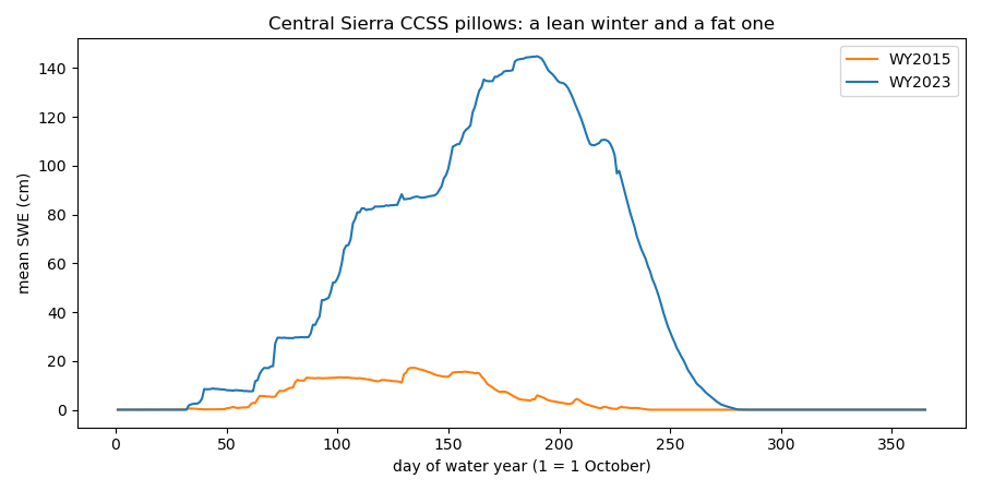
Two contrasting winters at the daily sites: 2015 (a record-low snowpack) and 2023 (a record-high one).

lean = esd.stations.load(daily, variables="swe", time="2014-10/2015-09")
fat = esd.stations.load(daily, variables="swe", time="2022-10/2023-09")

fig, ax = plt.subplots(figsize=(9, 4.5))
for label, obs, colour in (("WY2015", lean, "tab:orange"), ("WY2023", fat, "tab:blue")):
    basin_mean = obs["swe"].mean(dim="station")
    ax.plot(obs["dowy"], basin_mean, color=colour, label=label)
ax.set_xlabel("day of water year (1 = 1 October)")
ax.set_ylabel(f"mean SWE ({lean['swe'].attrs['units']})")
ax.set_title("Central Sierra CCSS pillows: a lean winter and a fat one")
ax.legend()
fig.tight_layout()

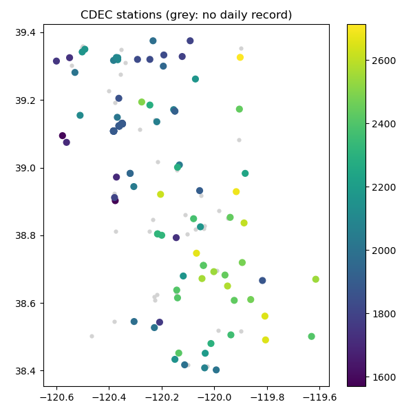
Where the stations sit, coloured by elevation.

fig, ax = plt.subplots(figsize=(6, 6))
everything.plot(ax=ax, color="lightgrey", markersize=12)
daily.plot(ax=ax, column="elevation_m", legend=True, markersize=40, cmap="viridis")
ax.set_title("CDEC stations (grey: no daily record)")
fig.tight_layout()