Köppen-Geiger classes, present and projected

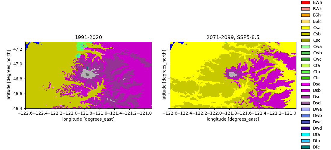
The Beck et al. (2023) classification at 1 km, and how the same box is projected to look at the end of the century under SSP5-8.5. The class table travels with the array as CF flag attributes, so the legend draws itself.

import matplotlib.pyplot as plt

import easysnowdata as esd

aoi = (-122.6, 46.4, -120.9, 47.3)  # Mount Rainier and its lowlands

Present-day classes (1991-2020, the default period).

present = esd.climate.koppen_geiger.load(aoi, resolution="1 km")
print(present.attrs["archive_member"], present.attrs["flag_meanings"][:40])

1991_2020/koppen_geiger_0p00833333.tif Af Am Aw BWh BWk BSh BSk Csa Csb Csc Cwa

The same box at the end of the century under SSP5-8.5.

future = esd.climate.koppen_geiger.load(
    aoi, period="2071_2099", scenario="ssp585", resolution="1 km"
)

fig, axes = plt.subplots(1, 2, figsize=(11, 5), sharey=True)
esd.plotting.categorical(present, ax=axes[0], legend=False, title="1991-2020")
esd.plotting.categorical(future, ax=axes[1], title="2071-2099, SSP5-8.5")
fig.tight_layout()

What the archive holds, without downloading it: every period, scenario and resolution is one row.

inventory = esd.climate.koppen_geiger.search()
print(inventory.head())
print(f"{len(inventory)} rasters in the archive")

      period scenario  ... resolution_m                                  member
0  1901_1930      NaN  ...     111000.0         1901_1930/koppen_geiger_1p0.tif
1  1901_1930      NaN  ...      55500.0         1901_1930/koppen_geiger_0p5.tif
2  1901_1930      NaN  ...      11100.0         1901_1930/koppen_geiger_0p1.tif
3  1901_1930      NaN  ...       1000.0  1901_1930/koppen_geiger_0p00833333.tif
4  1931_1960      NaN  ...     111000.0         1931_1960/koppen_geiger_1p0.tif

[5 rows x 5 columns]
72 rasters in the archive