CEAZA-Met snow stations (Coquimbo, Chile)

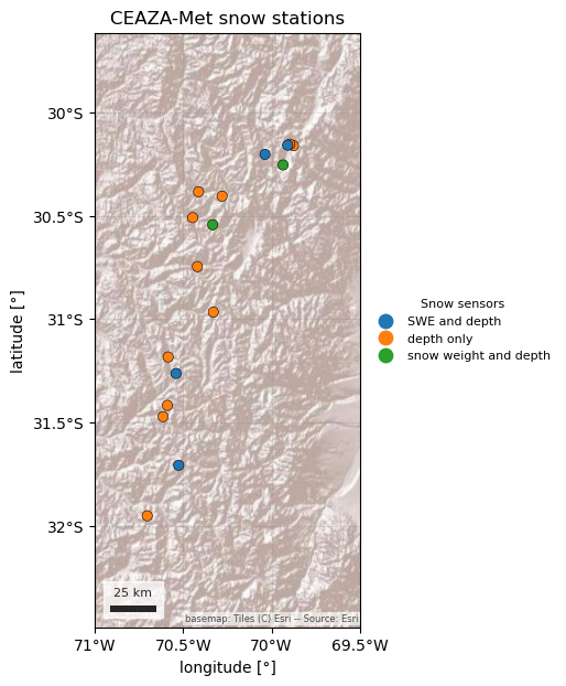
CEAZA-Met is the station network of the Centro de Estudios Avanzados en Zonas Áridas (CEAZA) in La Serena, Chile. Most of its roughly 95 stations are agricultural and coastal weather stations, but 17 high-Andes stations between 2,284 and 4,306 m, at 30–32° S, measure snow: all of them snow depth, and six also snow water equivalent, either as “Agua equivalente” (El Tapado, Tascadero, and the closed Hualtatas and La Laguna series) or as snow weight in kg/m² (Guandacol, Llano de Las Liebres). The values are raw logger output with no quality control.

CEAZAClient reads CEAZA-Met’s open web service. By default it lists only the snow stations and returns daily snow depth and SWE in cm. Air temperature and precipitation are there too, as non-default variables, and so are hourly values. Every record carries the code of the sensor that made it, because some stations have two sensors of the same kind. The terms of use ask you to register by e-mail with CEAZA and to credit “Datos provistos por el laboratorio de meteorología CEAZA” with a link to www.ceazamet.cl. It is not part of esd.stations.inventory() or load().

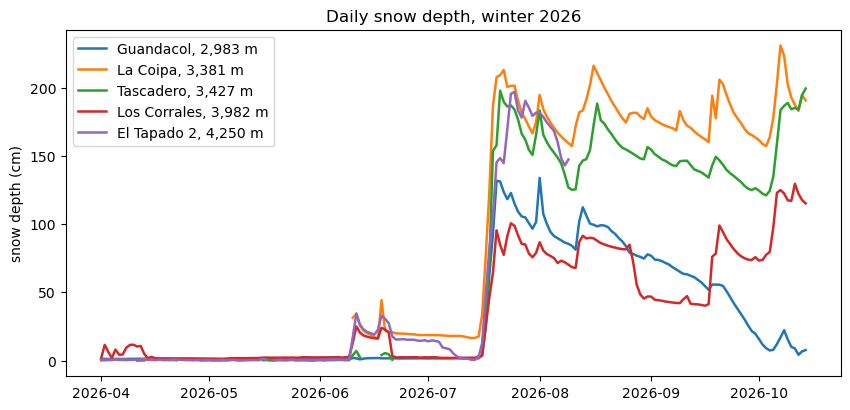
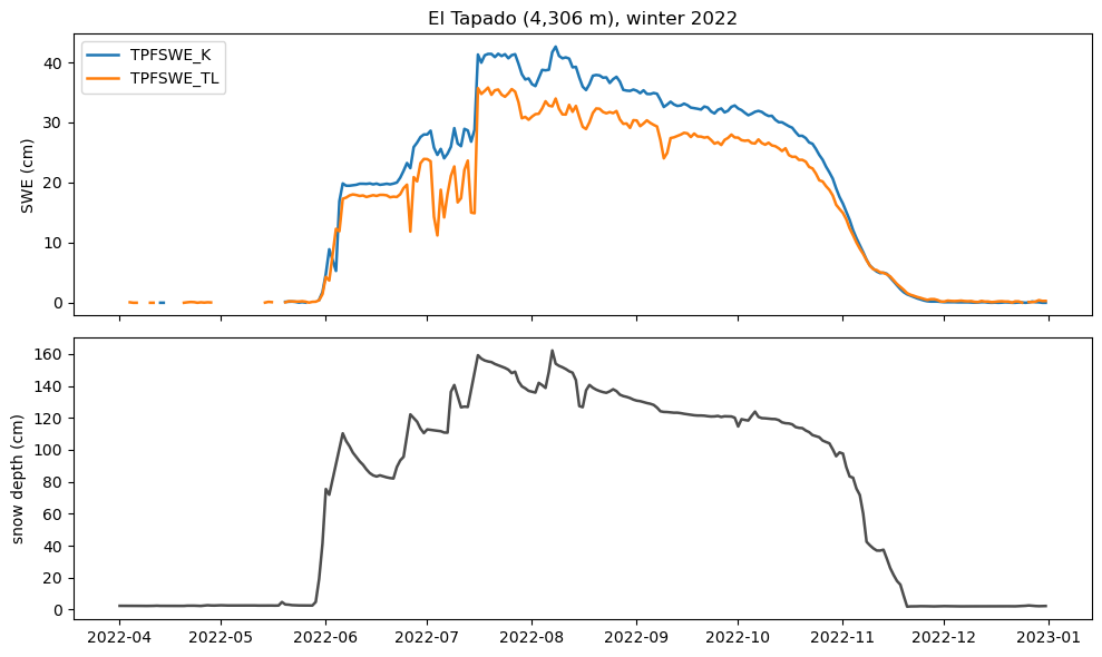
The figures show where the snow stations are and what they measure, snow depth through the 2026 winter at five elevations, and two SWE sensors at El Tapado (4,306 m) through the 2022 winter.

import geopandas as gpd
import matplotlib.pyplot as plt
import pandas as pd

import easysnowdata as esd
from easysnowdata.stations.clients import CEAZAClient

client = CEAZAClient()

The snow stations, coloured by the kind of snow sensor they have. A station is “Active” when its latest reading is at most 90 days old.

stations_df = pd.DataFrame(client.get_all_stations()).set_index("station_id")
stations_df["sensors"] = stations_df["snow_variables"].map(
    lambda v: (
        "SWE and depth"
        if {"ae_mm", "ae_cm"} & set(v)
        else "snow weight and depth"
        if "pnkg" in v
        else "depth only"
    )
)
print(
    stations_df[["name", "elevation_m", "status", "end_date", "sensors"]]
    .sort_values("elevation_m")
    .to_string()
)
stations_gdf = gpd.GeoDataFrame(
    stations_df,
    geometry=gpd.points_from_xy(stations_df["longitude"], stations_df["latitude"]),
    crs="EPSG:4326",
)
ax = esd.plotting.points(
    stations_gdf,
    column="sensors",
    legend_label="Snow sensors",
    title="CEAZA-Met snow stations",
    markersize=45,
    edgecolor="black",
    figsize=(7, 7),
    pad=0.3,
)
# The stations sit in a narrow north-south strip: pad the view so the edge
# stations are not clipped, and space the longitude labels so they fit.
lons = [-71.0, -70.5, -70.0, -69.5]
ax.set_xticks(lons, labels=[f"{-lon:g}°W" for lon in lons])

                             name  elevation_m    status    end_date                sensors
station_id
TRQ                    Tranquilla       2284.0  Inactive  2018-03-06             depth only
LAGHU              Laguna Hurtado       2500.0  Inactive  2025-09-13             depth only
LMBT        Los Molles [Bocatoma]       2543.0  Inactive  2025-04-12             depth only
EPLV                     El Polvo       2561.0  Inactive  2025-12-05             depth only
TQ                 Tres Quebradas       2812.0  Inactive  2019-03-18             depth only
HDC                     Guandacol       2983.0    Active  2026-10-21  snow weight and depth
EDER               Estero Derecho       3020.0    Active  2026-09-01             depth only
LAGEL           La Laguna [Elqui]       3209.0    Active  2026-10-21          SWE and depth
LCP                      La Coipa       3381.0    Active  2026-10-21             depth only
TASC                    Tascadero       3427.0    Active  2026-10-20          SWE and depth
LLL          Llano de Las Liebres       3565.0    Active  2026-10-21  snow weight and depth
CDC                Casa del Canto       3570.0    Active  2026-10-21             depth only
HUAL                    Hualtatas       3632.0  Inactive  2019-10-23          SWE and depth
EJT                       El Jote       3660.0    Active  2026-10-21             depth only
CORR                 Los Corrales       3982.0    Active  2026-10-21             depth only
TPF2                  El Tapado 2       4250.0    Active  2026-08-09             depth only
TPF                     El Tapado       4306.0  Inactive  2025-11-26          SWE and depth
/home/runner/work/easysnowdata/easysnowdata/docs/gallery/station_datasets/plot_ceaza.py:60: GeographicAxesWarning: The data are in a geographic CRS (EPSG:4326), so one axis unit is a degree, not a metre. The axes use a latitude-corrected aspect (1/cos(-31.1°) = 1.17) so shapes are not stretched; for a true equal-area grid load the product with crs='utm'.
  ax = esd.plotting.points(

[<matplotlib.axis.XTick object at 0x7fba94391590>, <matplotlib.axis.XTick object at 0x7fba82a3f750>, <matplotlib.axis.XTick object at 0x7fba82a3f610>, <matplotlib.axis.XTick object at 0x7fba6f944910>]

Daily mean snow depth through the 2026 winter, from Guandacol (2,983 m) to El Tapado 2 (4,250 m). On bare ground the sensors read close to zero; a day that reads below zero (the sensor’s offset) comes back as None and breaks the line. El Tapado 2 stops reporting in early August.

sites = {
    "HDC": "Guandacol, 2,983 m",
    "LCP": "La Coipa, 3,381 m",
    "TASC": "Tascadero, 3,427 m",
    "CORR": "Los Corrales, 3,982 m",
    "TPF2": "El Tapado 2, 4,250 m",
}
depth_df = pd.DataFrame(
    client.get_data(
        list(sites), variables="snwd", begin_date="2026-04-01", end_date="2026-10-14"
    )
).assign(date=lambda df: pd.to_datetime(df["date"]))
print(depth_df.groupby("station_id")["value"].agg(["count", "max"]).round(1))
fig, ax = plt.subplots(figsize=(10, 4.5))
for sid, label in sites.items():
    site = depth_df[depth_df["station_id"] == sid].set_index("date")["value"]
    site = site.asfreq("D")  # leave gaps where there is no value
    ax.plot(site.index, site.values, lw=1.8, label=label)
ax.set(ylabel="snow depth (cm)", title="Daily snow depth, winter 2026")
ax.legend(loc="upper left")

            count    max
station_id
CORR          197  129.6
HDC           197  133.9
LCP           165  230.9
TASC          140  199.4
TPF2          130  196.9

<matplotlib.legend.Legend object at 0x7fba6ff30a50>

El Tapado has two SWE sensors (TPFSWE_K and TPFSWE_TL, served in mm and returned in cm) beside a snow-depth sensor. In the 2022 winter both sensors pass 35 cm of SWE but disagree by several cm, which is why records keep the sensor code.

tapado_df = pd.DataFrame(
    client.get_data(
        "TPF",
        variables=["swe", "snwd"],
        sensors=["TPFSWE_K", "TPFSWE_TL", "TPFANSHM31"],
        begin_date="2022-04-01",
        end_date="2022-12-31",
    )
).assign(date=lambda df: pd.to_datetime(df["date"]))
fig, (ax_swe, ax_depth) = plt.subplots(2, 1, figsize=(10, 6), sharex=True)
for sensor in ["TPFSWE_K", "TPFSWE_TL"]:
    series = tapado_df[tapado_df["sensor"] == sensor].set_index("date")["value"]
    ax_swe.plot(series.index, series.values, lw=1.8, label=sensor)
ax_swe.set(ylabel="SWE (cm)", title="El Tapado (4,306 m), winter 2022")
ax_swe.legend(loc="upper left")
depth = tapado_df[tapado_df["sensor"] == "TPFANSHM31"].set_index("date")["value"]
ax_depth.plot(depth.index, depth.values, color="0.3", lw=1.8)
ax_depth.set(ylabel="snow depth (cm)")
fig.tight_layout()