German snow depth and SWE (DWD)

Deutscher Wetterdienst publishes daily snow depth from about 2,600 active climate and precipitation stations, and SWE from about 500, as open data (CC BY 4.0). SWE is manual: an observer cuts a snow core, mostly only when the snowpack is about 5 cm or deeper, so even in a snowy winter few stations have it on most days. Snow depth is the stronger product. The big summits’ SWE series ended when those stations went automatic (Feldberg, Arber, Fichtelberg, Brocken), but their snow depth continues.

DWDClient reads DWD’s open-data files, merging the quality-controlled historical files with the daily-updated recent ones. It is not part of esd.stations.inventory() or load().

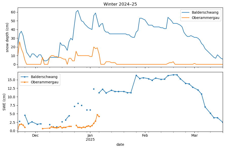
The figures show where SWE and snow-depth stations are, and one winter of snow depth and SWE at two stations at the foot of the Alps.

import geopandas as gpd
import matplotlib.pyplot as plt
import pandas as pd

import easysnowdata as esd
from easysnowdata.stations.clients import DWDClient

client = DWDClient()

Active stations, from both station lists. Every SWE station also measures snow depth.

stations = client.get_all_stations(active_only=True)
stations_gdf = gpd.GeoDataFrame(
    pd.DataFrame(stations).set_index("station_id"),
    geometry=gpd.points_from_xy(
        [s["longitude"] for s in stations], [s["latitude"] for s in stations]
    ),
    crs="EPSG:4326",
)
stations_gdf["reports"] = stations_gdf["has_swe"].map(
    {True: "SWE and snow depth", False: "snow depth"}
)
print(stations_gdf["reports"].value_counts().to_string())

ax = esd.plotting.points(
    stations_gdf,
    column="reports",
    legend_label="snow variables",
    title="Active DWD snow stations",
    markersize=3,
)

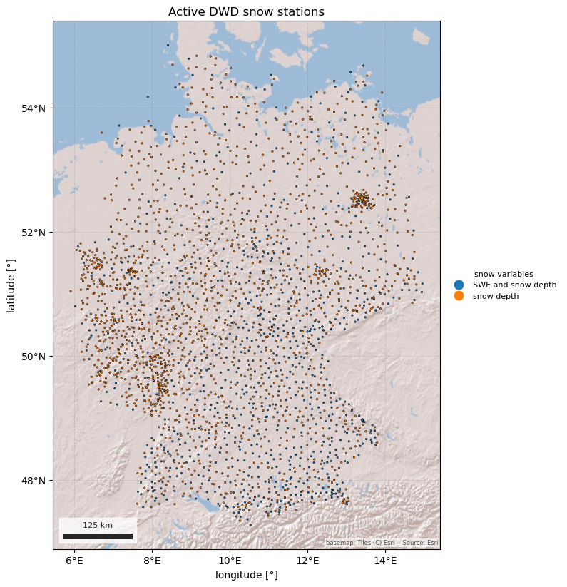
reports
snow depth            1767
SWE and snow depth     869
/home/runner/work/easysnowdata/easysnowdata/docs/gallery/station_datasets/plot_dwd.py:46: GeographicAxesWarning: The data are in a geographic CRS (EPSG:4326), so one axis unit is a degree, not a metre. The axes use a latitude-corrected aspect (1/cos(51.1°) = 1.59) so shapes are not stretched; for a true equal-area grid load the product with crs='utm'.
  ax = esd.plotting.points(

One winter at Balderschwang (1,039 m) in the Allgäu and Oberammergau (832 m) in the Ammergau Alps. SWE gaps are days without a core, not missing snow.

records = client.get_data(
    ["00275", "03677"],
    variables=["swe", "snwd"],
    begin_date="2024-11-01",
    end_date="2025-04-30",
)
obs_df = pd.DataFrame(records).assign(date=lambda df: pd.to_datetime(df["date"]))
fig, axes = plt.subplots(2, 1, figsize=(9, 6), sharex=True)
for ax, kind in zip(axes, ["snwd", "swe"], strict=True):
    wide_df = obs_df[obs_df["type"] == kind].pivot_table(
        index="date", columns="station_id", values="value"
    )
    wide_df.columns = [stations_gdf.loc[c, "name"] for c in wide_df.columns]
    wide_df.plot(ax=ax, marker="." if kind == "swe" else None)
    ax.set_ylabel(f"{'snow depth' if kind == 'snwd' else 'SWE'} (cm)")
axes[0].set_title("Winter 2024–25")
fig.tight_layout()