Note
Go to the end to download the full example code.
UCLA snow reanalysis (Margulis et al.)#
The UCLA snow reanalysis is a daily 480 m record of posterior snow water equivalent, snow depth and snow-covered area from a particle-batch smoother that assimilates Landsat fractional snow cover into an ensemble of snow model runs. Each variable comes with five ensemble statistics (mean, standard deviation, median, 25th and 75th percentiles), so the spread is part of the product.
Two regions from NSIDC, both behind Earthdata Login: region="wus" (the
default, WUS_UCLA_SR v1, water years 1985-2021 over the western United
States) and region="hma" (HMA_SR_D v1, water years 2000-2017 over
High Mountain Asia). The granules are one NetCDF-4 file per water year and
1 degree tile; past a handful of them virtualize="auto" switches to
cached kerchunk references.
The figures show SWE on 1 April 2020 over Mount Rainier, the water year of basin-mean SWE, and the ensemble spread around it.
import numpy as np

import easysnowdata as esd

aoi = (-121.94, 46.72, -121.54, 46.99)  # Mount Rainier, WA
water_year = "2019-10-01/2020-09-30"

box = esd.parse_aoi(aoi)
grid = box.to_geobox(crs="utm", resolution=500)  # the map below is drawn on this grid
print(box)
print(grid)
AOI(bounds=(-121.9400, 46.7200, -121.5400, 46.9900), clip=True)
GeoBox((62, 63), Affine(500.0, 0.0, 580500.0,
       0.0, -500.0, 5205500.0), CRS('EPSG:32610'))
Where the product comes from, and what each route asks for.
for src in esd.catalog.get("ucla-snow-reanalysis").sources:
    print(f"{src.id:22} {src.title:45} {', '.join(src.requires) or 'no account'}")
nsidc                  NSIDC (Earthdata)                             earthdata
nsidc-hma              NSIDC HMA (Earthdata)                         earthdata
One water year of the ensemble-mean SWE. A single granule is opened straight
through earthaccess.open, which the virtualized attribute records.
The box, loaded with a 1 km margin so the UTM grid is fully covered, is 366
days of about 65 by 95 pixels, under 10 MB, so it is pulled into memory once
and everything after this is instant.
swe_da = esd.snow.ucla_sr.load(box.buffer(1000), water_year).compute()
print(swe_da)
print(f"virtualized={swe_da.attrs['virtualized']}, access={swe_da.attrs['access']}")
<xarray.DataArray 'SWE_Post' (time: 366, latitude: 66, longitude: 97)> Size: 9MB
array([[[0.    , 0.    , 0.    , ..., 0.    , 0.    , 0.    ],
        [0.    , 0.    , 0.    , ..., 0.    , 0.    , 0.    ],
        [0.    , 0.    , 0.    , ..., 0.    , 0.    , 0.    ],
        ...,
        [0.    , 0.    , 0.    , ..., 0.    , 0.    , 0.    ],
        [0.    , 0.    , 0.    , ..., 0.    , 0.    , 0.    ],
        [0.    , 0.    , 0.    , ..., 0.    , 0.    , 0.    ]],

       [[0.    , 0.    , 0.    , ..., 0.    , 0.    , 0.    ],
        [0.    , 0.    , 0.    , ..., 0.    , 0.    , 0.    ],
        [0.    , 0.    , 0.    , ..., 0.    , 0.    , 0.    ],
        ...,
        [0.    , 0.    , 0.    , ..., 0.    , 0.    , 0.    ],
        [0.    , 0.    , 0.    , ..., 0.    , 0.    , 0.    ],
        [0.    , 0.    , 0.    , ..., 0.    , 0.    , 0.    ]],

       [[0.    , 0.    , 0.    , ..., 0.    , 0.    , 0.    ],
        [0.    , 0.    , 0.    , ..., 0.    , 0.    , 0.    ],
        [0.    , 0.    , 0.    , ..., 0.    , 0.    , 0.    ],
        ...,
...
        [0.    , 0.    , 0.    , ..., 0.    , 0.    , 0.    ],
        [0.    , 0.0006, 0.0202, ..., 0.    , 0.    , 0.    ],
        [0.    , 0.    , 0.0012, ..., 0.    , 0.    , 0.    ]],

       [[0.    , 0.    , 0.    , ..., 0.    , 0.    , 0.    ],
        [0.    , 0.    , 0.    , ..., 0.    , 0.    , 0.    ],
        [0.    , 0.    , 0.    , ..., 0.    , 0.    , 0.    ],
        ...,
        [0.    , 0.    , 0.    , ..., 0.    , 0.    , 0.    ],
        [0.    , 0.0006, 0.02  , ..., 0.    , 0.    , 0.    ],
        [0.    , 0.    , 0.0012, ..., 0.    , 0.    , 0.    ]],

       [[0.    , 0.    , 0.    , ..., 0.    , 0.    , 0.    ],
        [0.    , 0.    , 0.    , ..., 0.    , 0.    , 0.    ],
        [0.    , 0.    , 0.    , ..., 0.    , 0.    , 0.    ],
        ...,
        [0.    , 0.    , 0.    , ..., 0.    , 0.    , 0.    ],
        [0.    , 0.0006, 0.0182, ..., 0.    , 0.    , 0.    ],
        [0.    , 0.    , 0.001 , ..., 0.    , 0.    , 0.    ]]],
      shape=(366, 66, 97), dtype=float32)
Coordinates:
  * time         (time) datetime64[us] 3kB 2019-10-01 2019-10-02 ... 2020-09-30
  * latitude     (latitude) float32 264B 47.0 46.99 46.99 ... 46.72 46.71 46.71
  * longitude    (longitude) float32 388B -122.0 -121.9 -121.9 ... -121.5 -121.5
    spatial_ref  int64 8B 0
Attributes: (12/19)
    Units:                 meters
    source:                nsidc
    source_id:             nsidc
    source_title:          NSIDC (Earthdata)
    source_url:            https://nsidc.org/data/wus_ucla_sr/versions/1
    product_id:            ucla-snow-reanalysis
    ...                    ...
    statistic:             mean
    variable:              SWE_Post
    virtualized:           False
    access:                indirect
    long_name:             posterior snow water equivalent
    units:                 m
virtualized=False, access=indirect
SWE on 1 April 2020. Like SNODAS, the reanalysis never melts perennial ice out, so SWE over the summit ice cap grows year on year: the maximum in this box is over 100 m while the median is under 1 m. Those are the model’s values, passed through untouched, and the colour scale is capped so the seasonal snowpack around the mountain is visible.
april_da = swe_da.sel(time="2020-04-01")
print(f"median {float(april_da.median()):.2f} m, maximum {float(april_da.max()):.1f} m")
print(f"pixels above 10 m (the ice cap): {int((april_da > 10).sum())}")

ax = esd.plotting.map(
    april_da.odc.reproject(grid, resampling="bilinear"),
    cmap="Blues",
    vmin=0,
    vmax=3,
    title="ensemble-mean SWE, 2020-04-01",
)
ax.figure.tight_layout()
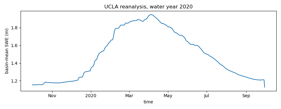
median 0.62 m, maximum 107.1 m
pixels above 10 m (the ice cap): 143
The water year as a basin mean over the seasonal snowpack only. A fixed cap leaves glacier pixels with a few metres of carried-over SWE in the mean, so the mask here is the water year itself: keep the pixels that melt out.
melts_out_da = swe_da.min(dim="time") < 0.01
print(
    f"pixels that melt out in the water year: {int(melts_out_da.sum())} of {melts_out_da.size}"
)
seasonal_da = swe_da.where(melts_out_da)
mean_da = seasonal_da.mean(dim=["latitude", "longitude"])
mean_da.attrs.update({"long_name": "basin-mean posterior SWE", "units": "m"})

ax = esd.plotting.timeseries(mean_da, color="tab:blue")
ax.set_ylim(bottom=0)
ax.figure.tight_layout()

peak_day = str(mean_da["time"].values[int(np.nanargmax(mean_da.values))])[:10]
print(f"peak basin-mean SWE {float(np.nanmax(mean_da.values)):.2f} m on {peak_day}")
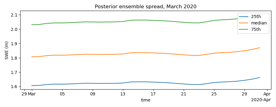
pixels that melt out in the water year: 5636 of 6402
peak basin-mean SWE 0.60 m on 2020-04-05
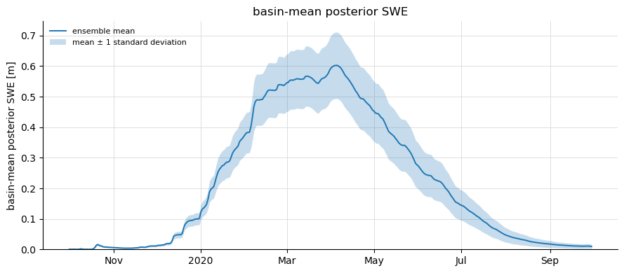
The ensemble spread: the same water year’s standard deviation, drawn as a band of one standard deviation around the mean.
std_da = esd.snow.ucla_sr.load(box.buffer(1000), water_year, stats="std").compute()
spread_da = std_da.where(melts_out_da).mean(dim=["latitude", "longitude"])

ax = esd.plotting.timeseries(mean_da, color="tab:blue", label="ensemble mean")
ax.fill_between(
    mean_da["time"].values,
    (mean_da - spread_da).values,
    (mean_da + spread_da).values,
    color="tab:blue",
    alpha=0.25,
    linewidth=0,
    label="mean ± 1 standard deviation",
)
ax.set_ylim(bottom=0)
ax.legend(fontsize=8, frameon=False, loc="upper left")
ax.figure.tight_layout()
The High Mountain Asia sibling is the same reanalysis over a different domain, and the same call reaches it:
hma_da = esd.snow.ucla_sr.load(
    (80.0, 30.0, 81.0, 31.0), "2000-10-01/2001-09-30", region="hma"
)
print(f"reference cache for long series: {esd.config.cache_dir('virtual', 'ucla_sr')}")
reference cache for long series: /home/runner/work/_temp/esd-cache/virtual/ucla_sr
Total running time of the script: (1 minutes 5.205 seconds)