Hillshade: Natural Earth shaded relief as a basemap

Natural Earth publishes global grayscale shaded relief in five styles, from a plain hillshade to “Gray Earth” with hypsometric tints, ocean-bottom relief and drainages, at 1 arcmin (the 1:10m scale) or 2 arcmin (1:50m). esd.terrain.hillshade.load fetches one style once into the easysnowdata cache and clips it to the AOI; with no AOI it returns the globe.

The values are cartographic brightness (0-255), not a physical quantity, so the layer belongs under other data rather than in an analysis. For a hillshade at DEM resolution, shade a DEM instead (see the DEM example).

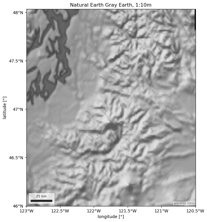
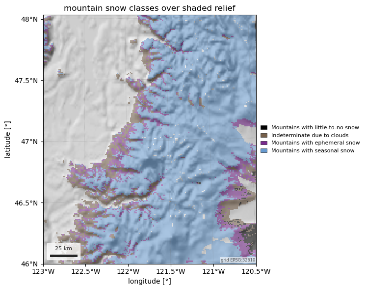
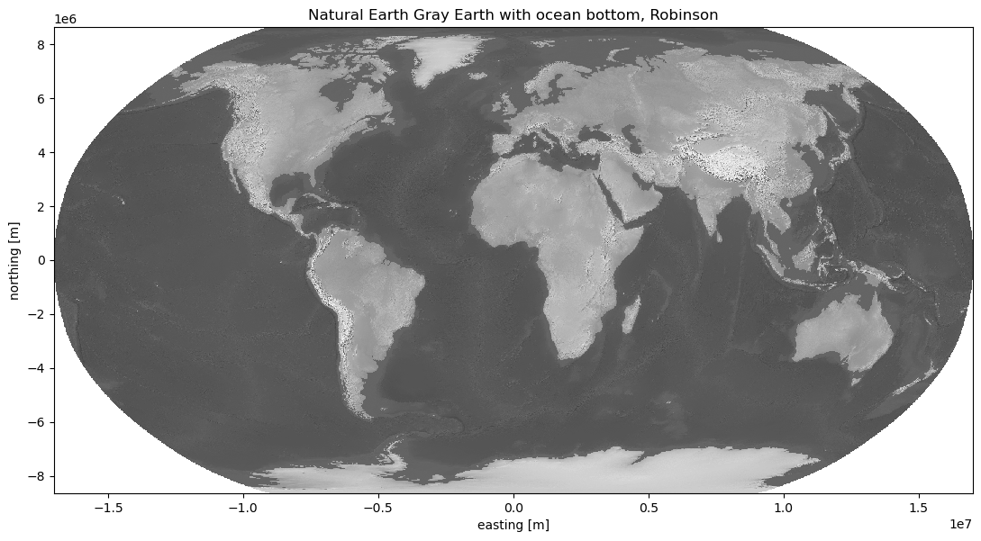
The figures show the default style over the central Cascades, the Wrzesien mountain snow mask drawn over it, and the whole globe in the Robinson projection the global snowmelt runoff onset maps use.

import matplotlib.pyplot as plt

import easysnowdata as esd

aoi = (-123.0, 46.0, -120.5, 48.0)  # the central Cascades, Puget Sound to Yakima

box = esd.parse_aoi(aoi)
grid = box.to_geobox(crs="utm", resolution=1000)  # the maps below share this grid
print(box)

AOI(bounds=(-123.0000, 46.0000, -120.5000, 48.0000), clip=True)

One route, no account; the style and scale choose the archive.

for src in esd.catalog.get("hillshade").sources:
    print(f"{src.id:15} {src.title:25} {', '.join(src.requires) or 'no account'}")
for style, (description, stems) in esd.terrain.hillshade.STYLES.items():
    print(f"{style:28} {', '.join(stems):8} {description}")

natural-earth   Natural Earth S3 bucket   no account
gray-earth-ocean-drainages   10m      Gray Earth with shaded relief, hypsography, ocean bottom, and drainages
gray-earth-ocean             10m, 50m Gray Earth with shaded relief, hypsography and ocean bottom
gray-earth-water             10m, 50m Gray Earth with shaded relief, hypsography and flat water
gray-earth                   10m, 50m Gray Earth with shaded relief and hypsography (land only)
shaded-relief                10m, 50m plain shaded relief

The default style, Gray Earth with ocean bottom and drainages at 1 arcmin (~1.85 km), resampled onto the AOI’s 1 km UTM grid. Puget Sound, the Columbia and the Cascade volcanoes are all legible at this scale.

hillshade_da = esd.terrain.hillshade.load(box.buffer(5000))
print(hillshade_da)

utm_hillshade_da = hillshade_da.odc.reproject(grid, resampling="bilinear")
ax = esd.plotting.map(
    utm_hillshade_da,
    cmap="gray",
    vmin=0,
    vmax=255,
    colorbar=False,
    title="Natural Earth Gray Earth, 1:10m",
)
ax.figure.tight_layout()

  0%|                                              | 0.00/91.7M [00:00<?, ?B/s]
  0%|                                      | 69.6k/91.7M [00:00<03:25, 445kB/s]
  0%|                                       | 279k/91.7M [00:00<01:34, 966kB/s]
  1%|▎                                     | 696k/91.7M [00:00<00:52, 1.74MB/s]
  2%|▌                                    | 1.48M/91.7M [00:00<00:27, 3.32MB/s]
  2%|▊                                    | 2.12M/91.7M [00:00<00:22, 4.03MB/s]
  4%|█▍                                   | 3.42M/91.7M [00:00<00:14, 6.17MB/s]
  5%|█▉                                   | 4.91M/91.7M [00:00<00:10, 8.21MB/s]
  8%|██▉                                  | 7.32M/91.7M [00:01<00:07, 11.9MB/s]
 11%|███▉                                 | 9.70M/91.7M [00:01<00:05, 14.5MB/s]
 15%|█████▌                               | 13.8M/91.7M [00:01<00:03, 20.5MB/s]
 20%|███████▍                             | 18.4M/91.7M [00:01<00:02, 27.3MB/s]
 24%|█████████                            | 22.4M/91.7M [00:01<00:02, 30.7MB/s]
 30%|██████████▉                          | 27.1M/91.7M [00:01<00:01, 35.4MB/s]
 36%|█████████████▏                       | 32.8M/91.7M [00:01<00:01, 39.0MB/s]
 41%|███████████████▎                     | 37.9M/91.7M [00:01<00:01, 40.9MB/s]
 48%|█████████████████▋                   | 43.8M/91.7M [00:01<00:01, 46.2MB/s]
 53%|███████████████████▋                 | 48.9M/91.7M [00:02<00:01, 42.3MB/s]
 58%|█████████████████████▍               | 53.2M/91.7M [00:02<00:00, 38.9MB/s]
 64%|███████████████████████▋             | 58.8M/91.7M [00:02<00:00, 43.2MB/s]
 70%|█████████████████████████▊           | 64.1M/91.7M [00:02<00:00, 41.5MB/s]
 76%|████████████████████████████▏        | 69.9M/91.7M [00:02<00:00, 45.9MB/s]
 83%|██████████████████████████████▌      | 75.9M/91.7M [00:02<00:00, 44.3MB/s]
 88%|████████████████████████████████▍    | 80.4M/91.7M [00:02<00:00, 40.8MB/s]
 94%|██████████████████████████████████▊  | 86.4M/91.7M [00:02<00:00, 45.5MB/s]
 99%|████████████████████████████████████▊| 91.1M/91.7M [00:03<00:00, 42.0MB/s]
  0%|                                              | 0.00/91.7M [00:00<?, ?B/s]
100%|██████████████████████████████████████| 91.7M/91.7M [00:00<00:00, 613GB/s]
<xarray.DataArray 'hillshade' (latitude: 126, longitude: 160)> Size: 20kB
dask.array<getitem, shape=(126, 160), dtype=uint8, chunksize=(126, 160), chunktype=numpy.ndarray>
Coordinates:
  * latitude     (latitude) float64 1kB 48.04 48.02 48.01 ... 45.99 45.97 45.96
  * longitude    (longitude) float64 1kB -123.1 -123.1 -123.0 ... -120.4 -120.4
    spatial_ref  int64 8B 0
Attributes: (12/14)
    source:                natural-earth
    source_id:             natural-earth
    source_title:          Natural Earth S3 bucket
    source_url:            https://naturalearth.s3.amazonaws.com/10m_raster/G...
    product_id:            hillshade
    title:                 Natural Earth global shaded relief (hillshade)
    ...                    ...
    easysnowdata_version:  0.3.3.dev40+g1bd7bbbf4
    style:                 gray-earth-ocean-drainages
    scale:                 1:10m
    file:                  GRAY_HR_SR_OB_DR.tif
    long_name:             shaded relief brightness (Gray Earth with shaded r...
    units:                 1

As a basemap: the plain shaded-relief style under the mountain snow mask’s seasonal and ephemeral classes, half transparent so the relief shows through where the classes are.

relief_da = esd.terrain.hillshade.load(box.buffer(5000), style="shaded-relief")
mask_da = esd.snow.mountain_snow_mask.load(box.buffer(5000), layer="mountain_snow")
utm_mask_da = mask_da.odc.reproject(grid, resampling="nearest")

fig, ax = plt.subplots(figsize=(8, 6))
esd.plotting.map(
    relief_da.odc.reproject(grid, resampling="bilinear"),
    ax=ax,
    cmap="gray",
    vmin=0,
    vmax=255,
    colorbar=False,
    scalebar=False,
    graticule=False,
)
esd.plotting.categorical(
    utm_mask_da.where(utm_mask_da != 255),  # Fill (not mountain) shows the relief
    ax=ax,
    alpha=0.55,
    title="mountain snow classes over shaded relief",
)
fig.tight_layout()

  0%|                                              | 0.00/44.4M [00:00<?, ?B/s]
  0%|                                      | 69.6k/44.4M [00:00<01:38, 451kB/s]
  0%|▏                                      | 157k/44.4M [00:00<01:25, 516kB/s]
  1%|▎                                      | 383k/44.4M [00:00<00:46, 948kB/s]
  2%|▋                                     | 801k/44.4M [00:00<00:26, 1.64MB/s]
  4%|█▎                                   | 1.57M/44.4M [00:00<00:15, 2.83MB/s]
  6%|██▏                                  | 2.65M/44.4M [00:00<00:09, 4.25MB/s]
 10%|███▌                                 | 4.32M/44.4M [00:01<00:06, 6.38MB/s]
 16%|█████▊                               | 6.94M/44.4M [00:01<00:03, 9.73MB/s]
 25%|█████████▏                           | 10.9M/44.4M [00:01<00:02, 16.6MB/s]
 33%|████████████▏                        | 14.7M/44.4M [00:01<00:01, 21.2MB/s]
 42%|███████████████▌                     | 18.7M/44.4M [00:01<00:00, 26.1MB/s]
 51%|███████████████████                  | 22.8M/44.4M [00:01<00:00, 30.0MB/s]
 65%|████████████████████████             | 28.9M/44.4M [00:01<00:00, 36.5MB/s]
 78%|████████████████████████████▉        | 34.7M/44.4M [00:01<00:00, 40.3MB/s]
 91%|█████████████████████████████████▋   | 40.4M/44.4M [00:01<00:00, 44.6MB/s]
  0%|                                              | 0.00/44.4M [00:00<?, ?B/s]
100%|██████████████████████████████████████| 44.4M/44.4M [00:00<00:00, 243GB/s]

The whole globe at 1:50m, reprojected to Robinson (ESRI:54030) at 20 km. This is the step the runoff-onset notebook does with gdalwarp; for a figure, reprojecting in memory is enough. rio.reproject (GDAL’s warper) rather than odc.reproject, because odc cannot trace the outline of a grid that reaches the poles in Robinson; pixels outside the projection’s outline are filled with 255 and masked.

world_da = esd.terrain.hillshade.load(scale="50m", style="gray-earth-ocean")
robinson_da = world_da.rio.reproject("ESRI:54030", resolution=20_000, nodata=255)
robinson_da = robinson_da.where(robinson_da != 255)
print(robinson_da.sizes)

ax = esd.plotting.map(
    robinson_da,
    cmap="gray",
    vmin=0,
    vmax=255,
    colorbar=False,
    scalebar=False,
    graticule=False,  # the edge labels would fall outside the Robinson outline
    title="Natural Earth Gray Earth with ocean bottom, Robinson",
    figsize=(11, 6),
)
ax.figure.tight_layout()

  0%|                                              | 0.00/24.8M [00:00<?, ?B/s]
  0%|                                      | 69.6k/24.8M [00:00<00:54, 452kB/s]
  1%|▎                                      | 191k/24.8M [00:00<00:37, 650kB/s]
  2%|▊                                     | 505k/24.8M [00:00<00:18, 1.28MB/s]
  4%|█▍                                    | 940k/24.8M [00:00<00:12, 1.89MB/s]
  7%|██▌                                  | 1.74M/24.8M [00:00<00:07, 3.08MB/s]
 13%|████▊                                | 3.19M/24.8M [00:00<00:04, 5.21MB/s]
 24%|████████▉                            | 6.02M/24.8M [00:01<00:01, 9.50MB/s]
 43%|███████████████▋                     | 10.5M/24.8M [00:01<00:00, 15.8MB/s]
 66%|████████████████████████▍            | 16.4M/24.8M [00:01<00:00, 25.4MB/s]
 85%|███████████████████████████████▍     | 21.0M/24.8M [00:01<00:00, 29.6MB/s]
  0%|                                              | 0.00/24.8M [00:00<?, ?B/s]
100%|██████████████████████████████████████| 24.8M/24.8M [00:00<00:00, 138GB/s]
Frozen({'y': 863, 'x': 1701})