PlanetScope beside Sentinel-2, and the UDM2 snow band

Output from the last scheduled build

This example needs planet credentials. The figures and printed output below come from the most recent scheduled build, which has them; this build reused that output instead of re-running the example.

PlanetScope is 3 m and near-daily, which is what makes it useful for catching a melt event between Sentinel-2 overpasses. It is also commercial: an order spends the account’s quota, so the ordering cell below is manual and does not run when the gallery is built.

Searching is free, so that part runs anywhere Planet credentials exist.

import matplotlib.pyplot as plt

import easysnowdata as esd

aoi = (-121.80, 46.82, -121.72, 46.88)
when = "2023-07-01/2023-07-03"

Search: free, and it only returns scenes the account may download.

scenes = esd.optical.planetscope.search(
    aoi, when, cloud_cover=20, asset_types=["ortho_analytic_4b_sr", "ortho_udm2"]
)
print(scenes[["acquired", "cloud_percent", "clear_percent", "snow_ice_percent"]])

                                                acquired  ...  snow_ice_percent
20230703_180548_93_2455 2023-07-03 18:05:48.931508+00:00  ...                21
20230703_180551_04_2455 2023-07-03 18:05:51.045197+00:00  ...                11
20230703_184655_52_2473 2023-07-03 18:46:55.521337+00:00  ...                 5
20230703_184657_65_2473 2023-07-03 18:46:57.652433+00:00  ...                22
20230701_180931_56_24b0 2023-07-01 18:09:31.566153+00:00  ...                14
20230701_180933_91_24b0 2023-07-01 18:09:33.917506+00:00  ...                12
20230701_184407_40_2477 2023-07-01 18:44:07.403272+00:00  ...                11
20230701_184405_26_2477 2023-07-01 18:44:05.266513+00:00  ...                22
20230701_180512_23_241f 2023-07-01 18:05:12.238603+00:00  ...                 8

[9 rows x 4 columns]

Warning

This cell spends Planet quota. It is the only step that does, and it is why load never orders by itself. Uncomment it to run it by hand. The clip tool means Planet charges for the AOI, not for the whole 600 MB strip; harmonize puts the radiometry on Sentinel-2’s scale.

order = esd.optical.planetscope.order(
    aoi,
    items=scenes.head(1),
    bundle="analytic_sr",
    harmonize="Sentinel-2",
)
ps = esd.optical.planetscope.load(aoi, order=order)

With a delivery in hand, the bands are named, the UDM2 mask is decoded into its layers, and the snow band is directly usable:

ndsi_like = esd.processing.normalized_difference(ps["green"], ps["nir"])
snow = ps["snow"]                       # UDM2 snow mask, 0/1
print(float(esd.optical.planetscope.snow_fraction(ps).isel(time=0)))

fig, axes = plt.subplots(1, 3, figsize=(14, 4.5))
esd.plotting.rgb(
    esd.processing.stretch_percentile(
        esd.processing.rgb(ps.isel(time=0), ("red", "green", "blue"))
    ),
    ax=axes[0],
    title="PlanetScope 3 m",
)
ndsi_like.isel(time=0).plot.imshow(ax=axes[1], cmap="Blues")
esd.plotting.categorical(snow.isel(time=0), ax=axes[2], title="UDM2 snow")

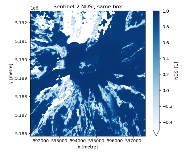
The free comparison: the same box from Sentinel-2, which needs no account and no quota. Run the Planet cells above to put the 3 m and 10 m views side by side.

s2 = esd.optical.sentinel2.load(
    aoi, when, bands=["green", "swir16", "red", "blue", "scl"], mask="scl-default"
)
ndsi = esd.processing.ndsi(s2)
if ndsi.sizes["time"]:
    fig, ax = plt.subplots(figsize=(6, 5))
    ndsi.isel(time=0).plot.imshow(ax=ax, cmap="Blues", vmin=-0.5, vmax=1.0)
    ax.set_title("Sentinel-2 NDSI, same box")
    ax.set_aspect("equal")
    fig.tight_layout()