SNODAS: the authoritative archive against the Earth Engine mirror

SNODAS now defaults to the NSIDC G02158 archive, which needs no account at all: one tar per day of flat-binary grids, read straight into xarray. The Climate Engine mirror on Earth Engine stays available and is faster for long series. They should agree, and this example checks that they do.

import matplotlib.pyplot as plt
import numpy as np

import easysnowdata as esd

aoi = (-121.94, 46.72, -121.54, 46.99)
when = ("2024-03-10", "2024-03-16")

The credential-free route. search lists the days and where each one lives, without downloading anything.

print(esd.snow.snodas.search(aoi, when).to_string())

swe = esd.snow.snodas.load(aoi, when)
print(swe)

        date                                                                                 url
0 2024-03-10  https://noaadata.apps.nsidc.org/NOAA/G02158/masked/2024/03_Mar/SNODAS_20240310.tar
1 2024-03-11  https://noaadata.apps.nsidc.org/NOAA/G02158/masked/2024/03_Mar/SNODAS_20240311.tar
2 2024-03-12  https://noaadata.apps.nsidc.org/NOAA/G02158/masked/2024/03_Mar/SNODAS_20240312.tar
3 2024-03-13  https://noaadata.apps.nsidc.org/NOAA/G02158/masked/2024/03_Mar/SNODAS_20240313.tar
4 2024-03-14  https://noaadata.apps.nsidc.org/NOAA/G02158/masked/2024/03_Mar/SNODAS_20240314.tar
5 2024-03-15  https://noaadata.apps.nsidc.org/NOAA/G02158/masked/2024/03_Mar/SNODAS_20240315.tar
6 2024-03-16  https://noaadata.apps.nsidc.org/NOAA/G02158/masked/2024/03_Mar/SNODAS_20240316.tar
<xarray.Dataset> Size: 91kB
Dimensions:      (time: 7, latitude: 33, longitude: 49)
Coordinates:
  * time         (time) datetime64[us] 56B 2024-03-10 2024-03-11 ... 2024-03-16
  * latitude     (latitude) float64 264B 46.99 46.98 46.97 ... 46.74 46.73 46.72
  * longitude    (longitude) float64 392B -121.9 -121.9 -121.9 ... -121.5 -121.5
    spatial_ref  int64 8B 0
Data variables:
    snow_depth   (time, latitude, longitude) float32 45kB dask.array<chunksize=(1, 33, 49), meta=np.ndarray>
    SWE          (time, latitude, longitude) float32 45kB dask.array<chunksize=(1, 33, 49), meta=np.ndarray>
Attributes:
    cache_dir:             /home/runner/.cache/easysnowdata/snodas
    source:                nsidc
    source_id:             nsidc
    source_title:          NSIDC G02158 (direct)
    source_url:            https://nsidc.org/data/g02158/versions/1
    product_id:            snodas
    title:                 SNODAS snow water equivalent and snow depth
    data_citation:         National Operational Hydrologic Remote Sensing Cen...
    license:               Public domain (US government data)
    easysnowdata_version:  0.0.27.dev125+g480e638d6
    doi:                   10.7265/N5TB14TC
    region:                masked

One day of SWE and snow depth.

fig, axes = plt.subplots(1, 2, figsize=(11, 4.5), sharey=True)
swe["SWE"].isel(time=0).plot.imshow(ax=axes[0], cmap="Blues", vmin=0, vmax=3)
axes[0].set_title("SNODAS SWE (m)")
swe["snow_depth"].isel(time=0).plot.imshow(ax=axes[1], cmap="Purples", vmin=0, vmax=8)
axes[1].set_title("SNODAS snow depth (m)")
for ax in axes:
    ax.set_aspect("equal")
fig.tight_layout()

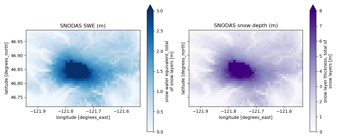
SNODAS never melts perennial ice out, so SWE grows without bound over glaciers and saturates the 16-bit field at 32.767 m. On Rainier that is the summit ice cap, and it is the model’s own behaviour rather than a reader artefact, so the values are passed through untouched. Mask them when a basin contains glaciers.

glaciated = swe["SWE"].isel(time=0) > 30
print(f"pixels saturated by the glacier artefact: {int(glaciated.sum())}")
seasonal = swe["SWE"].where(swe["SWE"] < 30)
print(f"median SWE without them: {float(np.nanmedian(seasonal.isel(time=0))):.2f} m")

pixels saturated by the glacier artefact: 9
median SWE without them: 0.78 m

The same week from the Earth Engine mirror, for users who already have an Earth Engine account and want a server-side subset:

mirror = esd.snow.snodas.load(aoi, when, source="gee-climate-engine")
both = xr.concat(
    [swe["SWE"].mean(dim=["latitude", "longitude"]),
     mirror["SWE"].mean(dim=["latitude", "longitude"])],
    dim="source",
)
both.plot(hue="source")

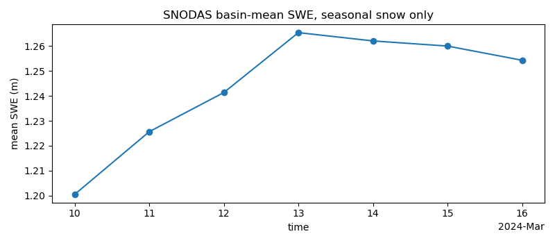
basin_mean = seasonal.mean(dim=["latitude", "longitude"]).compute()
fig, ax = plt.subplots(figsize=(8, 3.5))
basin_mean.plot(ax=ax, marker="o")
ax.set_ylabel("mean SWE (m)")
ax.set_title("SNODAS basin-mean SWE, seasonal snow only")
fig.tight_layout()