Argentine snow pillows (SNIH)

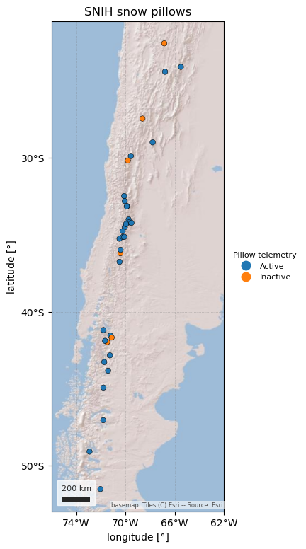
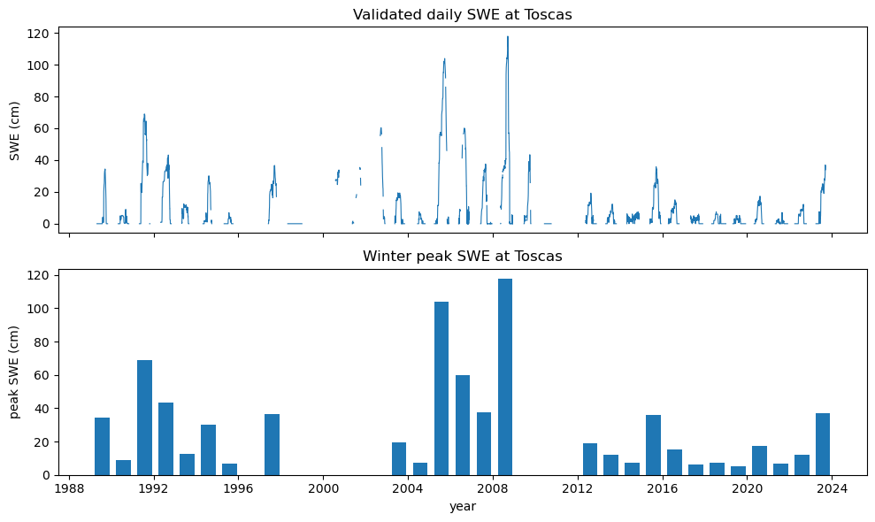
Argentina’s Sistema Nacional de Información Hídrica (SNIH), run by the Secretaría de Infraestructura y Política Hídrica, publishes the country’s hydrometeorological records, including 34 snow pillows along the Andes from Jujuy (24° S) to Santa Cruz (52° S). The five pillows of the Mendoza Andes have validated daily SWE from 1989–1999 onward and snow-course surveys from 1951; the others are newer, and the pillows of the RMET network (from 2024) have only raw telemetry so far.

SNIHClient talks to the portal’s own JSON page methods (no account is needed). It returns three separate products, never mixed: validated daily pillow SWE (interval="daily"), raw pillow telemetry every 4 or 6 hours ("sub_daily", flagged "raw") and snow-course surveys ("periodic"). Values are in cm, dates in Argentina time. The portal’s terms allow any use, including commercial, if you cite SIPH and the network, keep the data’s meaning and state the date of the last update. It is not part of esd.stations.inventory() or load().

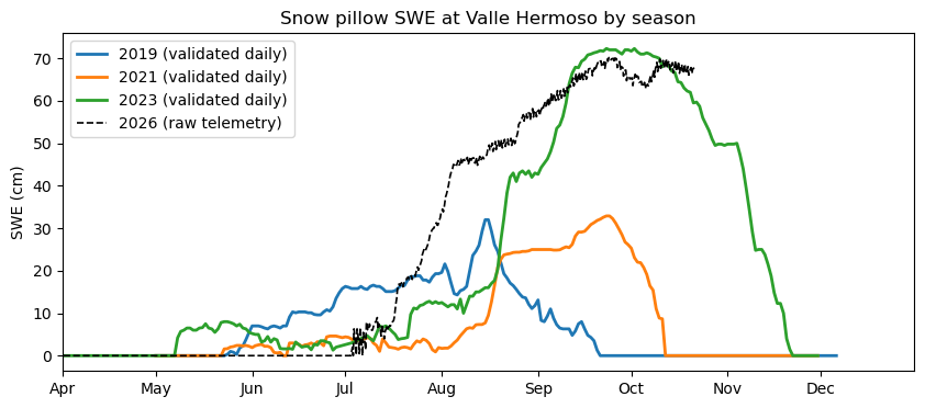
The figures show where the pillows are, the 35-year validated record at Toscas above Mendoza, and this winter’s raw telemetry at Valle Hermoso next to earlier validated seasons.

import geopandas as gpd
import matplotlib.pyplot as plt
import pandas as pd

import easysnowdata as esd
from easysnowdata.stations.clients import SNIHClient

client = SNIHClient()

The snow stations. The client keeps the 50 stations the portal links to a snow parameter; 34 have a pillow. “Active” means the pillow sent data in the last 30 days.

stations_df = pd.DataFrame(client.get_all_stations()).set_index("station_id")
pillows_df = stations_df[stations_df["has_swe"]]
print(
    pillows_df.groupby(["network", "status"]).size().unstack(fill_value=0).to_string()
)
pillows_gdf = gpd.GeoDataFrame(
    pillows_df,
    geometry=gpd.points_from_xy(pillows_df["longitude"], pillows_df["latitude"]),
    crs="EPSG:4326",
)
ax = esd.plotting.points(
    pillows_gdf,
    column="status",
    legend_label="Pillow telemetry",
    title="SNIH snow pillows",
    markersize=30,
    edgecolor="black",
    figsize=(6, 9),
)
# The Andes are long and thin: widen the view so the labels have room.
ax.set_xlim(-76, -62)
lons = [-74, -70, -66, -62]
ax.set_xticks(lons, labels=[f"{-lon}°W" for lon in lons])

status                    Active  Inactive
network
Red Hidrológica Nacional      20         4
Red Meteorológica RMET         9         2
/home/runner/work/easysnowdata/easysnowdata/docs/gallery/station_datasets/plot_snih.py:50: GeographicAxesWarning: The data are in a geographic CRS (EPSG:4326), so one axis unit is a degree, not a metre. The axes use a latitude-corrected aspect (1/cos(-37.0°) = 1.25) so shapes are not stretched; for a true equal-area grid load the product with crs='utm'.
  ax = esd.plotting.points(

[<matplotlib.axis.XTick object at 0x7fba82a3fc50>, <matplotlib.axis.XTick object at 0x7fba6ff32c10>, <matplotlib.axis.XTick object at 0x7fba6ff33ed0>, <matplotlib.axis.XTick object at 0x7fba6f969bd0>]

Toscas (2,950 m, upper Mendoza basin): every validated daily SWE value since 1989, and each winter’s peak. Winters with fewer than 100 days of data are left out of the peaks. The validated series ends in 2023.

toscas_df = pd.DataFrame(client.get_data("19145")).assign(
    date=lambda df: pd.to_datetime(df["date"])
)
print(toscas_df["interval"].unique(), len(toscas_df), "days")
winters = toscas_df.groupby(toscas_df["date"].dt.year)["value"].agg(["max", "count"])
peaks = winters[winters["count"] >= 100]["max"]
# Missing days become gaps in the line rather than straight joins.
toscas_daily = toscas_df.set_index("date")["value"].asfreq("D")
fig, (ax1, ax2) = plt.subplots(2, 1, figsize=(10, 6), sharex=True)
ax1.plot(toscas_daily.index, toscas_daily.values, lw=0.8)
ax1.set(ylabel="SWE (cm)", title="Validated daily SWE at Toscas")
ax2.bar(pd.to_datetime(peaks.index.astype(str) + "-08-01"), peaks.values, width=250)
ax2.set(xlabel="year", ylabel="peak SWE (cm)", title="Winter peak SWE at Toscas")
fig.tight_layout()

<ArrowStringArray>
['daily']
Length: 1, dtype: str 5301 days

Valle Hermoso (2,253 m, Río Grande): three validated winters and the current one. 2026 has no validated values yet, so it is the raw 6-hourly telemetry, drawn dashed: it has not been checked and can jump.

seasons = [2019, 2021, 2023]
daily_df = pd.DataFrame(
    client.get_data("19121", begin_date="2019-04-01", end_date="2023-12-31")
).assign(date=lambda df: pd.to_datetime(df["date"]))
raw_df = pd.DataFrame(
    client.get_data(
        "19121", interval="sub_daily", begin_date="2026-04-01", end_date="2026-12-31"
    )
).assign(time=lambda df: pd.to_datetime(df["datetime"], utc=True))
print(raw_df[["datetime", "value"]].tail(3).to_string(index=False))

fig, ax = plt.subplots(figsize=(10, 4))
for year in seasons:
    season = daily_df[daily_df["date"].dt.year == year]
    day = season["date"].dt.dayofyear
    ax.plot(day, season["value"], lw=2, label=f"{year} (validated daily)")
raw_day = raw_df["time"].dt.tz_convert("America/Argentina/Mendoza")
ax.plot(
    raw_day.dt.dayofyear + raw_day.dt.hour / 24,
    raw_df["value"],
    "k--",
    lw=1.2,
    label="2026 (raw telemetry)",
)
months = pd.date_range("2021-04-01", "2021-12-01", freq="MS")
ax.set_xticks(months.dayofyear, labels=months.strftime("%b"))
ax.set_xlim(months[0].dayofyear, months[-1].dayofyear + 30)
ax.set(ylabel="SWE (cm)", title="Snow pillow SWE at Valle Hermoso by season")
ax.legend()

                 datetime  value
2026-10-20T12:00:00-03:00 66.401
2026-10-20T18:00:00-03:00 67.400
2026-10-21T06:00:00-03:00 67.816

<matplotlib.legend.Legend object at 0x7fb9fa276fd0>