NLCD land cover, annual (USGS)

The National Land Cover Database maps the conterminous United States at 30 m in sixteen classes. The official release is frozen at the 2001-2021 epochs; Annual NLCD (collection 1) redid the whole record as one map per year from 1985 to 2024, so land cover can be followed through time instead of compared between two epochs.

Both routes are on Earth Engine and need esd.auth.login("earthengine"): source="gee-annual" (default) is the community mirror of Annual NLCD, source="gee" the official 2021 release with its science products and impervious-surface descriptors. The class table is read from the asset at run time and attached as CF flags, so esd.plotting.categorical draws the USGS palette.

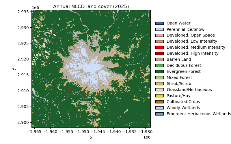
The first figure is the first and the last year of the record side by side. The second follows the area of the main classes through all forty years: the Cascades’ evergreen forest is a patchwork of clear-cuts and regrowth, and the annual record shows the shrub and grass that appear where a stand was cut and the forest that returns twenty years later.

import matplotlib.pyplot as plt

import easysnowdata as esd

aoi = (-121.94, 46.72, -121.54, 46.99)  # Mount Rainier, WA

box = esd.parse_aoi(aoi)
grid = box.to_geobox(crs="utm", resolution=30)  # every map below is drawn on this grid
print(box)
print(grid)

AOI(bounds=(-121.9400, 46.7200, -121.5400, 46.9900), clip=True)
GeoBox((1017, 1033), Affine(30.0, 0.0, 580590.0,
       0.0, -30.0, 5205090.0), CRS('EPSG:32610'))

Where the product comes from: two Earth Engine assets, both need an account.

for src in esd.catalog.get("nlcd").sources:
    print(f"{src.id:22} {src.title:45} {', '.join(src.requires) or 'no account'}")

gee-annual             Earth Engine (Annual NLCD)                    earthengine
gee                    Earth Engine (2021 release)                   earthengine

The whole annual record for the box: one 30 m map per year on the asset’s native Albers grid, 40 years in one lazy array. Selecting a year gives a 2-D map that keeps its date as a scalar coordinate. The box is loaded with a 1 km margin so the AOI’s UTM grid the maps use is fully covered; the class areas below are counted on the native Albers pixels.

landcover_da = esd.land.nlcd.load(box.buffer(1000), time="1985/2024")
print(landcover_da)
first_da, last_da = landcover_da.isel(time=0), landcover_da.isel(time=-1)

fig, axes = plt.subplots(1, 2, figsize=(14, 5.8), layout="constrained")
esd.plotting.categorical(
    first_da.odc.reproject(grid, resampling="nearest"),
    ax=axes[0],
    legend=False,
    title="Annual NLCD 1985",
)
esd.plotting.categorical(
    last_da.odc.reproject(grid, resampling="nearest"),
    ax=axes[1],
    title="Annual NLCD 2024",
)

<xarray.DataArray 'landcover' (time: 40, y: 1301, x: 1319)> Size: 69MB
array([[[42, 42, 42, ..., 52, 52, 52],
        [42, 42, 42, ..., 52, 71, 71],
        [42, 42, 42, ..., 52, 42, 42],
        ...,
        [71, 71, 52, ..., 42, 42, 42],
        [71, 71, 52, ..., 42, 42, 42],
        [71, 71, 71, ..., 42, 42, 42]],

       [[42, 42, 42, ..., 52, 52, 52],
        [42, 42, 42, ..., 52, 71, 71],
        [42, 42, 42, ..., 52, 42, 42],
        ...,
        [71, 71, 52, ..., 42, 42, 42],
        [71, 71, 52, ..., 42, 42, 42],
        [71, 71, 71, ..., 42, 42, 42]],

       [[42, 42, 42, ..., 52, 52, 52],
        [42, 42, 42, ..., 52, 71, 71],
        [42, 42, 42, ..., 52, 42, 42],
        ...,
...
        [42, 52, 52, ..., 42, 42, 42],
        [42, 52, 52, ..., 42, 42, 42],
        [42, 52, 52, ..., 42, 42, 42]],

       [[42, 42, 42, ..., 52, 52, 52],
        [42, 42, 42, ..., 52, 42, 42],
        [42, 42, 42, ..., 42, 42, 42],
        ...,
        [42, 52, 52, ..., 42, 42, 42],
        [42, 52, 52, ..., 42, 42, 42],
        [42, 52, 52, ..., 42, 42, 42]],

       [[42, 42, 42, ..., 52, 52, 52],
        [42, 42, 42, ..., 52, 42, 42],
        [42, 42, 42, ..., 42, 42, 42],
        ...,
        [42, 52, 52, ..., 42, 42, 42],
        [42, 52, 52, ..., 42, 42, 42],
        [42, 52, 52, ..., 42, 42, 42]]],
      shape=(40, 1301, 1319), dtype=uint8)
Coordinates:
  * time         (time) datetime64[ms] 320B 1985-01-01 1986-01-01 ... 2024-01-01
  * y            (y) float64 10kB 2.936e+06 2.936e+06 ... 2.897e+06 2.897e+06
  * x            (x) float64 11kB -1.967e+06 -1.967e+06 ... -1.927e+06
    spatial_ref  int64 8B 0
Attributes: (12/23)
    id:                    b1
    data_type:             {'type': 'PixelType', 'precision': 'int', 'min': 0...
    dimensions:            [160000, 105000]
    crs_transform:         [30, 0, -2415585, 0, -30, 3314805]
    flag_values:           [11, 12, 21, 22, 23, 24, 31, 41, 42, 43, 52, 71, 8...
    flag_meanings:         Open_Water Perennial_Ice/Snow Developed,_Open_Spac...
    ...                    ...
    license:               Public domain (US government data)
    easysnowdata_version:  0.3.9.dev1+gd97689c2f
    doi:                   10.5066/P9JZ7AO3
    asset:                 projects/sat-io/open-datasets/USGS/ANNUAL_NLCD/LAN...
    layer:                 landcover
    extent:                CONUS

<Axes: title={'center': 'Annual NLCD 2024'}, xlabel='longitude [°]', ylabel='latitude [°]'>

Class area through time, as the change since 1985. A pixel is 900 m², so a class count per year is an area. Most of the box is Mount Rainier National Park, which is not logged, but the national forest around it was clear-cut heavily before the 1990s: the shrub/scrub of those cuts shrinks year by year as the stands close back into evergreen forest, and the two curves are close to mirror images. Perennial ice/snow does not move at all.

classes_df = esd.processing.categorical.flags(landcover_da).set_index("value")
follow = {
    42: "Evergreen forest",
    52: "Shrub/scrub",
    71: "Grassland/herbaceous",
    12: "Perennial ice/snow",
}
fig, ax = plt.subplots(figsize=(9, 4.2))
for value, name in follow.items():
    area_km2_da = (landcover_da == value).sum(dim=("y", "x")) * 900 / 1e6
    print(
        f"{name:22} {float(area_km2_da.isel(time=0)):7.1f} km² in 1985, "
        f"{float(area_km2_da.isel(time=-1)):7.1f} km² in 2024"
    )
    ax.plot(
        landcover_da["time"].values,
        (area_km2_da - area_km2_da.isel(time=0)).values,
        label=name,
        color=classes_df.loc[value, "color"],
        linewidth=1.8,
    )
ax.axhline(0, color="0.3", linewidth=0.8)
ax.set_ylabel("area change since 1985 [km²]")
ax.set_title("Annual NLCD class area, change since 1985")
ax.grid(True, color="0.85", linewidth=0.6)
ax.set_axisbelow(True)
for side in ("top", "right"):
    ax.spines[side].set_visible(False)
ax.legend(frameon=False, fontsize=9)
fig.tight_layout()

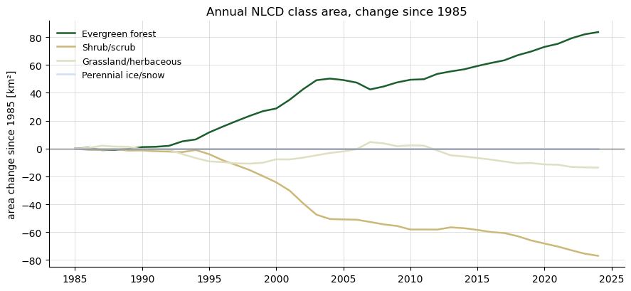
Evergreen forest        1092.5 km² in 1985,  1176.1 km² in 2024
Shrub/scrub              187.3 km² in 1985,   110.3 km² in 2024
Grassland/herbaceous      22.4 km² in 1985,     8.7 km² in 2024
Perennial ice/snow        72.8 km² in 1985,    72.8 km² in 2024