ESA WorldCover land cover

ESA WorldCover is a global 10 m land cover map in eleven classes, made from Sentinel-1 and Sentinel-2 for 2020 (version="v100") and 2021 (version="v200", the default and the last one the project produced). The classes come back as CF flag_values / flag_meanings / flag_colors attributes, so esd.plotting.categorical draws the map in the product’s own palette with a legend of the classes present.

Both routes are credential-free: the Planetary Computer STAC collection (source="planetary-computer", the default) and the unsigned AWS Open Data bucket (source="aws-open-data"), which reads the 3°×3° tiles directly.

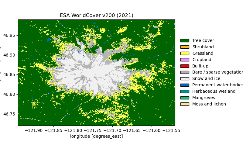
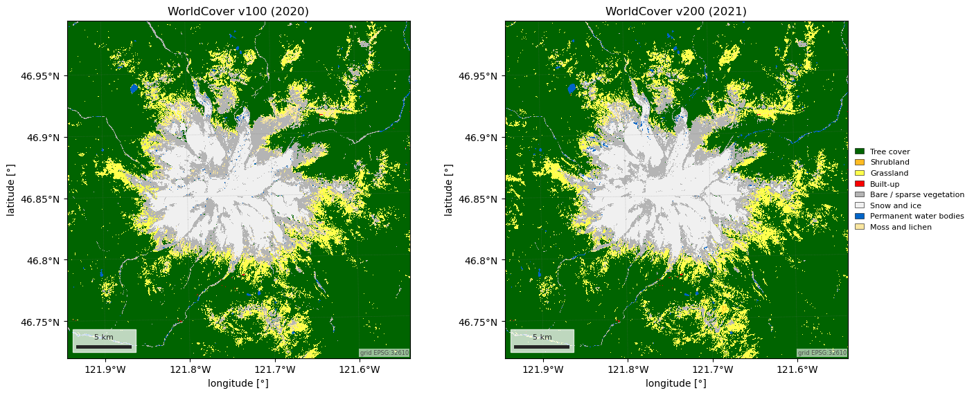
The first figure is the 2021 map on a UTM grid, with the area of each class. The second puts 2020 next to 2021: ESA’s own guidance is that the two versions were made with different algorithms and are not a change product, and the fraction of pixels that flip between them says why.

import matplotlib.pyplot as plt
import numpy as np
import pandas as pd

import easysnowdata as esd

aoi = (-121.94, 46.72, -121.54, 46.99)  # Mount Rainier, WA

esd.parse_aoi(aoi)  # the AOI as every loader below will see it

AOI(bounds=(-121.9400, 46.7200, -121.5400, 46.9900), clip=True)

Where the product comes from: two routes, neither needs an account.

for src in esd.catalog.get("esa-worldcover").sources:
    print(f"{src.id:22} {src.title:45} {', '.join(src.requires) or 'no account'}")

planetary-computer     Planetary Computer                            no account
aws-open-data          AWS Open Data bucket                          no account

The 2021 map on the AOI’s UTM zone at the native 10 m, so a pixel is 100 m² and class areas are a count. Tree cover fills the valleys and stops at the treeline; above it WorldCover sees bare rock, snow and ice, and a ring of grassland in the subalpine meadows between.

landcover_da = esd.land.landcover.load(aoi, crs="utm", grid_resolution=10, chunks=None)
print(landcover_da)
esd.plotting.categorical(landcover_da, title="ESA WorldCover v200 (2021)")

classes_df = esd.processing.categorical.flags(landcover_da)
values, counts = np.unique(landcover_da.values, return_counts=True)
area = pd.Series(counts * 100 / 1e6, index=values).rename("area [km²]")
table_df = classes_df.set_index("value")["meaning"].str.replace("_", " ").to_frame()
table_df = table_df.join(area, how="inner").sort_values("area [km²]", ascending=False)
print(table_df.round(1).to_string())

<xarray.DataArray 'landcover' (y: 3050, x: 3098)> Size: 9MB
array([[10, 10, 10, ..., 10, 10, 10],
       [10, 10, 10, ..., 10, 10, 10],
       [10, 10, 10, ..., 10, 10, 10],
       ...,
       [10, 10, 10, ..., 10, 10, 10],
       [10, 10, 10, ..., 10, 10, 10],
       [10, 10, 10, ..., 10, 10, 10]], shape=(3050, 3098), dtype=uint8)
Coordinates:
  * y            (y) float64 24kB 5.205e+06 5.205e+06 ... 5.175e+06 5.175e+06
  * x            (x) float64 25kB 5.806e+05 5.806e+05 ... 6.116e+05 6.116e+05
    time         datetime64[us] 8B 2021-01-01
    spatial_ref  int64 8B 0
Attributes: (12/18)
    nodata:                0
    _FillValue:            0
    source:                planetary-computer
    source_id:             planetary-computer
    source_title:          Planetary Computer
    source_url:            https://planetarycomputer.microsoft.com/api/stac/v...
    ...                    ...
    version:               v200
    year:                  2021
    long_name:             land cover class
    flag_values:           [10, 20, 30, 40, 50, 60, 70, 80, 90, 95, 100]
    flag_meanings:         Tree_cover Shrubland Grassland Cropland Built-up B...
    flag_colors:           #006400 #FFBB22 #FFFF4C #F096FF #FA0000 #B4B4B4 #F...
                        meaning  area [km²]
value
10                   Tree cover       650.5
70                 Snow and ice        99.3
30                    Grassland        95.4
60     Bare / sparse vegetation        81.7
100             Moss and lichen        12.4
80       Permanent water bodies         5.2
20                    Shrubland         0.3
50                     Built-up         0.1

2020 (v100) against 2021 (v200). The versions differ in algorithm as well as in year, so the pixels that change class between them are mostly a change of method, not of land. The largest flips are between neighbouring classes: tree cover against grassland, in both directions, along the treeline, and the alpine classes (moss and lichen, bare ground, snow and ice) against each other on the mountain, where which one wins depends on the summer scenes each version saw.

earlier_da = esd.land.landcover.load(
    aoi, version="v100", crs="utm", grid_resolution=10, chunks=None
)
names = classes_df.set_index("value")["meaning"].str.replace("_", " ")
flips_df = pd.DataFrame(
    {"v100": earlier_da.values.ravel(), "v200": landcover_da.values.ravel()}
)
flips_df = flips_df[flips_df["v100"] != flips_df["v200"]]
print(
    f"pixels that change class between v100 and v200: {len(flips_df) / landcover_da.size:.1%}"
)
top = flips_df.value_counts().head(6).rename("area [km²]") * 100 / 1e6
top.index = [f"{names[a]} -> {names[b]}" for a, b in top.index]
print(top.round(1).to_string())

fig, axes = plt.subplots(1, 2, figsize=(14, 5.6), layout="constrained")
esd.plotting.categorical(
    earlier_da, ax=axes[0], legend=False, title="WorldCover v100 (2020)"
)
esd.plotting.categorical(landcover_da, ax=axes[1], title="WorldCover v200 (2021)")

pixels that change class between v100 and v200: 8.4%
Tree cover -> Grassland                        16.3
Grassland -> Tree cover                        10.7
Moss and lichen -> Grassland                   10.4
Bare / sparse vegetation -> Snow and ice        8.7
Bare / sparse vegetation -> Grassland           5.7
Moss and lichen -> Bare / sparse vegetation     5.2

<Axes: title={'center': 'WorldCover v200 (2021)'}, xlabel='longitude [°]', ylabel='latitude [°]'>