Hydro-Québec gamma SWE sensors (live feed)

Hydro-Québec runs about 95 passive-gamma (GMON) SWE sensors across its hydropower basins, the largest network of automated SWE outside SNOTEL in North America. Its open-data portal serves hourly SWE, snow depth and weather from these and its other stations, with no account, under CC BY-NC 4.0 (attribution, no commercial reuse).

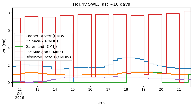
The feed holds only the last ~10 days. HydroQuebecClient reads that window; anything older must be accumulated by whoever calls it, and CanSWE carries the GMON history up to the last snow season. SWE rows are hourly but the sensor value changes every 6 hours. interval="daily" aggregates over the local (Eastern) day: the last value of the day for SWE and depth, sums for precipitation, means for the rest.

It is not part of esd.stations.inventory() or load().

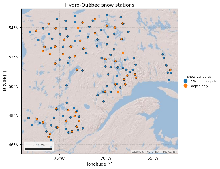
The figures show the snow stations in the current window and the hourly and daily SWE of the stations that have snow right now. Out of season the feed mostly shows zeros.

import geopandas as gpd
import pandas as pd

import easysnowdata as esd
from easysnowdata.stations.clients import HydroQuebecClient

client = HydroQuebecClient()

Stations with SWE or snow depth in the current window.

stations = client.get_all_stations()
stations_gdf = gpd.GeoDataFrame(
    pd.DataFrame(stations).set_index("station_id"),
    geometry=gpd.points_from_xy(
        [s["longitude"] for s in stations], [s["latitude"] for s in stations]
    ),
    crs="EPSG:4326",
)
stations_gdf["reports"] = stations_gdf["has_swe"].map(
    {True: "SWE and depth", False: "depth only"}
)
print(stations_gdf["reports"].value_counts().to_string())
print(f"window: {stations_gdf['begin_date'].min()} to {stations_gdf['end_date'].max()}")

ax = esd.plotting.points(
    stations_gdf,
    column="reports",
    legend_label="snow variables",
    title="Hydro-Québec snow stations",
)

reports
SWE and depth    96
depth only       48
window: 2026-10-11 to 2026-10-21
/home/runner/work/easysnowdata/easysnowdata/docs/gallery/station_datasets/plot_hydroquebec.py:49: GeographicAxesWarning: The data are in a geographic CRS (EPSG:4326), so one axis unit is a degree, not a metre. The axes use a latitude-corrected aspect (1/cos(50.3°) = 1.57) so shapes are not stretched; for a true equal-area grid load the product with crs='utm'.
  ax = esd.plotting.points(

Hourly SWE for every GMON station in the window, then the daily values.

swe_ids = list(stations_gdf.index[stations_gdf["has_swe"]])
hourly_df = pd.DataFrame(client.get_data(swe_ids, variables="swe", interval="hourly"))
daily_df = pd.DataFrame(client.get_data(swe_ids, variables="swe", interval="daily"))
print(f"{len(hourly_df)} hourly and {len(daily_df)} daily SWE records")

22961 hourly and 1045 daily SWE records

The five stations with the highest SWE right now, hourly, in UTC. Note the 6-hourly steps. Out of season, as in October, non-zero values at stations whose snow depth is 0 are sensor noise rather than snow.

latest = hourly_df.dropna(subset=["value"]).groupby("station_id")["value"].last()
top = latest.sort_values(ascending=False).index[:5]
wide_df = (
    hourly_df[hourly_df["station_id"].isin(top)]
    .assign(time=lambda df: pd.to_datetime(df["datetime"]))
    .pivot_table(index="time", columns="station_id", values="value")
)
wide_df.columns = [stations_gdf.loc[c, "name"] for c in wide_df.columns]
ax = wide_df.plot(
    figsize=(9, 4), drawstyle="steps-post", title="Hourly SWE, last ~10 days"
)
ax.set_ylabel("SWE (cm)")

Text(23.999999999999993, 0.5, 'SWE (cm)')