Countries, states, counties and admin units

esd.boundaries.admin answers “which country, state, county or district is this?” with four products:

• countries() — Natural Earth at 1:110m, 1:50m or 1:10m, or geoBoundaries ADM0;

• states() — states and provinces worldwide from Natural Earth, US states from the Census Bureau (picked automatically for a US AOI), or geoBoundaries ADM1;

• counties() — US counties from the Census Bureau;

• admin() — any level (ADM0-ADM5) of any country from geoBoundaries.

Each returns a GeoDataFrame in EPSG:4326 whose first columns are name, iso3 and admin_level, whatever the source, and each archive is fetched once into the easysnowdata cache. None of them needs an account.

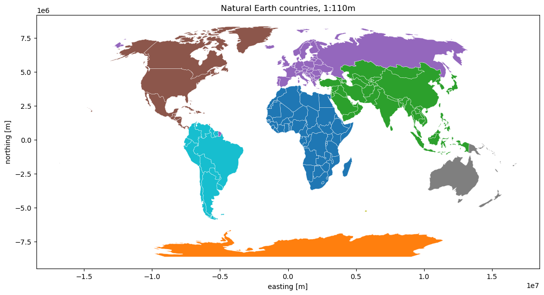
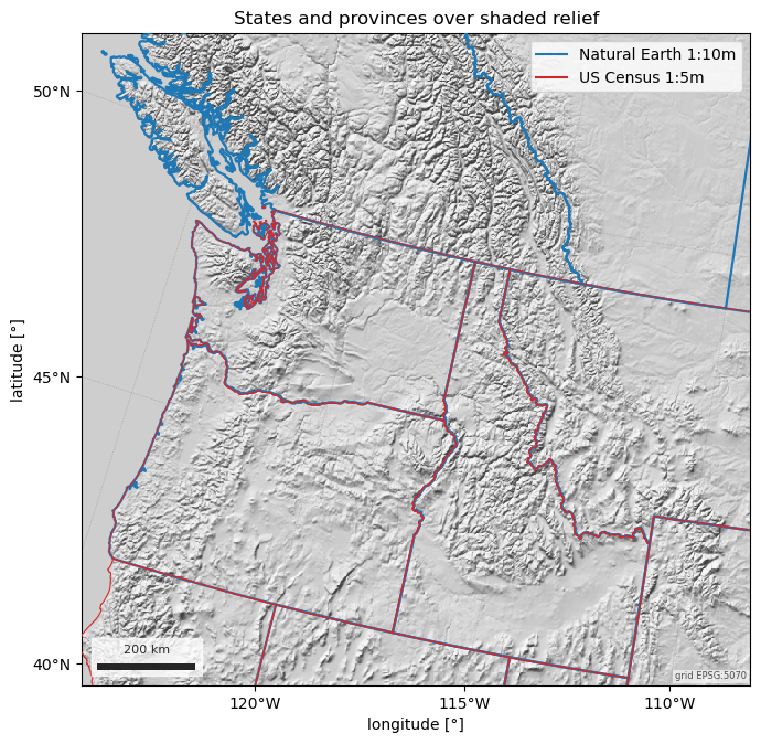
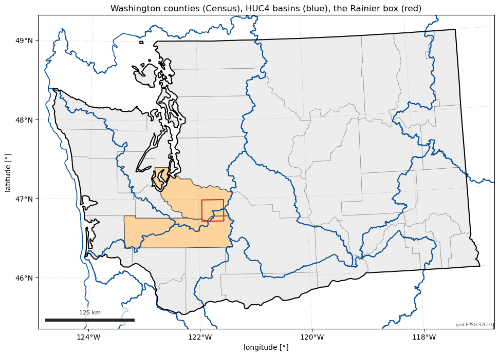
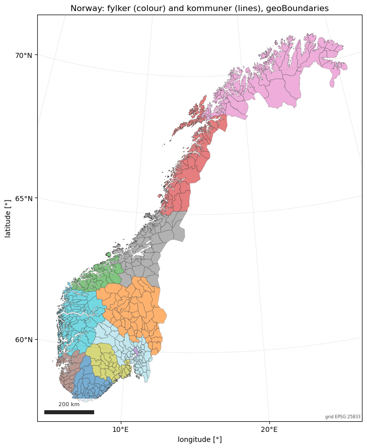
The figures show the world, the Pacific Northwest’s states and provinces over the Natural Earth hillshade, Washington’s counties with the HUC4 basins a state polygon selects when it is used as an AOI, and Norway’s counties and municipalities from geoBoundaries.

import matplotlib.pyplot as plt

import easysnowdata as esd

rainier = (-121.94, 46.72, -121.54, 46.99)  # Mount Rainier, WA

Where each product comes from, and what the route asks for.

for product_id in ("countries", "states-provinces", "us-counties", "admin-boundaries"):
    for src in esd.catalog.get(product_id).sources:
        print(
            f"{product_id:18} {src.id:14} {src.title:34} {', '.join(src.requires) or 'no account'}"
        )

countries          natural-earth  Natural Earth                      no account
countries          geoboundaries  geoBoundaries (gbOpen)             no account
states-provinces   natural-earth  Natural Earth                      no account
states-provinces   us-census      US Census cartographic boundaries  no account
states-provinces   geoboundaries  geoBoundaries (gbOpen)             no account
us-counties        us-census      US Census cartographic boundaries  no account
admin-boundaries   geoboundaries  geoBoundaries (gbOpen)             no account

The world at 1:110m, Natural Earth’s default for a map this size, coloured by continent and drawn in Robinson.

world_gdf = esd.boundaries.admin.countries()
print(f"{len(world_gdf)} countries; columns start with {list(world_gdf.columns[:3])}")
print(world_gdf.loc[world_gdf["iso3"].isin(["NOR", "FRA"]), ["name", "iso3", "ISO_A3"]])

robinson = "ESRI:54030"
ax = world_gdf.to_crs(robinson).plot(
    column="CONTINENT", cmap="tab10", edgecolor="white", linewidth=0.3, figsize=(11, 6)
)
esd.plotting.finish_map(ax, robinson, scalebar=False, graticule=False)
ax.set_title("Natural Earth countries, 1:110m")
ax.figure.tight_layout()

  0%|                                               | 0.00/215k [00:00<?, ?B/s]
  0%|                                               | 0.00/215k [00:00<?, ?B/s]
100%|███████████████████████████████████████| 215k/215k [00:00<00:00, 1.63GB/s]
177 countries; columns start with ['name', 'iso3', 'admin_level']
      name iso3 ISO_A3
21  Norway  NOR    -99
43  France  FRA    -99

The ISO_A3 column above is -99 for Norway and France, a Natural Earth quirk; iso3 comes from ADM0_A3 and is always set.

States and provinces across the Pacific Northwest. The AOI straddles the border, so states() reads Natural Earth’s first-level units for both countries; restricted to the US, it switches to the Census Bureau’s cartographic boundaries, which are the authoritative US outlines. The two are drawn over the Natural Earth hillshade, on one Albers grid.

pnw = (-125.0, 42.0, -110.0, 52.0)
grid = esd.parse_aoi(pnw).to_geobox(crs="EPSG:5070", resolution=2000)

ne_states_gdf = esd.boundaries.admin.states(pnw)
census_states_gdf = esd.boundaries.admin.states(pnw, country="USA")
print(ne_states_gdf[["name", "iso3", "admin_level"]].to_string(index=False))
print(census_states_gdf.attrs["source"], census_states_gdf.attrs["resolution"])

# The Albers grid's corners reach beyond the lon/lat box, so the hillshade is
# read with a margin that covers them.
hillshade_da = esd.terrain.hillshade.load(
    (-130.0, 38.0, -104.0, 56.0), style="shaded-relief"
)
ax = esd.plotting.map(
    hillshade_da.odc.reproject(grid, resampling="bilinear"),
    cmap="gray",
    vmin=0,
    vmax=255,
    colorbar=False,
    title="States and provinces over shaded relief",
)
esd.plotting.add_outline(ax, ne_states_gdf, edgecolor="#1f77b4", linewidth=1.6)
esd.plotting.add_outline(ax, census_states_gdf, edgecolor="#d62728", linewidth=0.8)
ax.plot([], [], color="#1f77b4", label="Natural Earth 1:10m")
ax.plot([], [], color="#d62728", label="US Census 1:5m")
ax.legend(loc="upper right")
ax.figure.tight_layout()

  0%|                                              | 0.00/14.9M [00:00<?, ?B/s]
 62%|███████████████████████              | 9.30M/14.9M [00:00<00:00, 93.0MB/s]
  0%|                                              | 0.00/14.9M [00:00<?, ?B/s]
100%|█████████████████████████████████████| 14.9M/14.9M [00:00<00:00, 89.2GB/s]

  0%|                                              | 0.00/1.12M [00:00<?, ?B/s]
  0%|                                              | 0.00/1.12M [00:00<?, ?B/s]
100%|█████████████████████████████████████| 1.12M/1.12M [00:00<00:00, 7.22GB/s]
            name iso3  admin_level
      Washington  USA            1
British Columbia  CAN            1
           Idaho  USA            1
         Montana  USA            1
         Alberta  CAN            1
          Oregon  USA            1
            Utah  USA            1
         Wyoming  USA            1
          Nevada  USA            1
us-census 1:5m

Washington’s 39 counties, with the two that contain Rainier picked out by AOI. A boundary is itself an AOI: the Washington polygon selects the HUC4 subregions it touches, from the USGS WBD service.

wa_counties_gdf = esd.boundaries.admin.counties(state="WA")
rainier_counties_gdf = esd.boundaries.admin.counties(rainier)
washington_gdf = esd.boundaries.admin.states(name="Washington", country="USA")
huc4_gdf = esd.hydro.basins.huc(washington_gdf, level=4)
print(rainier_counties_gdf[["name", "STUSPS", "GEOID"]].to_string(index=False))
print(huc4_gdf[["huc4", "name"]].to_string(index=False))

utm = esd.parse_aoi(washington_gdf).utm_crs
fig, ax = plt.subplots(figsize=(10, 7))
wa_counties_gdf.to_crs(utm).plot(ax=ax, color="0.93", edgecolor="0.55", linewidth=0.5)
rainier_counties_gdf.to_crs(utm).plot(ax=ax, color="#fdd49e", edgecolor="0.3")
huc4_gdf.to_crs(utm).boundary.plot(ax=ax, color="#08519c", linewidth=1.2)
washington_gdf.to_crs(utm).boundary.plot(ax=ax, color="black", linewidth=1.5)
esd.parse_aoi(rainier).to_crs(utm).boundary.plot(ax=ax, color="#d62728", linewidth=1.5)
b = washington_gdf.to_crs(utm).total_bounds
ax.set_xlim(b[0] - 20_000, b[2] + 20_000)
ax.set_ylim(b[1] - 20_000, b[3] + 20_000)
esd.plotting.finish_map(ax, utm)
ax.set_title("Washington counties (Census), HUC4 basins (blue), the Rainier box (red)")
fig.tight_layout()

  0%|                                              | 0.00/2.98M [00:00<?, ?B/s]
  0%|                                              | 0.00/2.98M [00:00<?, ?B/s]
100%|█████████████████████████████████████| 2.98M/2.98M [00:00<00:00, 20.3GB/s]
  name STUSPS GEOID
 Lewis     WA 53041
Pierce     WA 53053
huc4                          name
1702                Upper Columbia
1711                   Puget Sound
1703                        Yakima
1706                   Lower Snake
1710     Oregon-Washington Coastal
1701 Kootenai-Pend Oreille-Spokane
1707               Middle Columbia
1708                Lower Columbia
1709                    Willamette

Any level of any country through geoBoundaries. Norway’s first level is its counties (fylker; the release holds the 11 of 2020-2023, before the 2024 split back to 15) and its second its municipalities (kommuner); simplified=True reads geoBoundaries’ lighter geometries. Every unit carries the licence of the national source it came from.

fylker_gdf = esd.boundaries.admin.admin(country="NOR", level=1, simplified=True)
kommuner_gdf = esd.boundaries.admin.admin(country="NOR", level=2, simplified=True)
print(f"{len(fylker_gdf)} fylker, {len(kommuner_gdf)} kommuner")
print(kommuner_gdf["boundaryLicense"].unique())

norway_utm = "EPSG:25833"
ax = fylker_gdf.to_crs(norway_utm).plot(
    column="name", cmap="tab20", alpha=0.6, edgecolor="none", figsize=(8, 9)
)
kommuner_gdf.to_crs(norway_utm).boundary.plot(ax=ax, color="0.25", linewidth=0.2)
esd.plotting.finish_map(ax, norway_utm)
ax.set_title("Norway: fylker (colour) and kommuner (lines), geoBoundaries")
ax.figure.tight_layout()

  0%|                                              | 0.00/3.22M [00:00<?, ?B/s]
  0%|                                              | 0.00/3.22M [00:00<?, ?B/s]
100%|█████████████████████████████████████| 3.22M/3.22M [00:00<00:00, 16.6GB/s]

  0%|                                              | 0.00/4.72M [00:00<?, ?B/s]
 89%|█████████████████████████████████    | 4.23M/4.72M [00:00<00:00, 42.3MB/s]
  0%|                                              | 0.00/4.72M [00:00<?, ?B/s]
100%|█████████████████████████████████████| 4.72M/4.72M [00:00<00:00, 33.3GB/s]
11 fylker, 431 kommuner
<ArrowStringArray>
['Creative Commons Attribution 4.0 International (CC BY 4.0)']
Length: 1, dtype: str