Southern Andes daily snow depth (Chile and Argentina)#

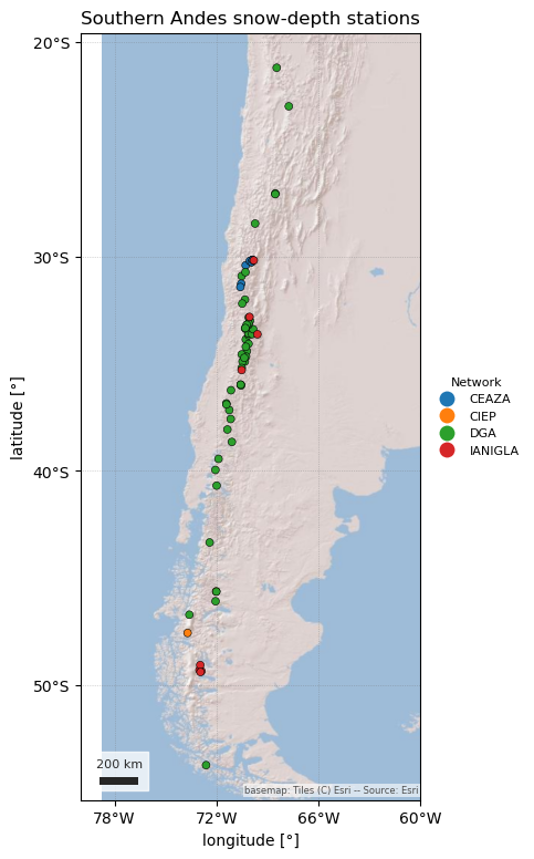
The Southern Andes Daily Snow Depth Dataset (Medina Mendoza & Caro, 2026; Caro et al., 2026, ESSD) compiles 69 automatic snow-depth stations from 21° S to 54° S, run by Chile’s Dirección General de Aguas (DGA), IANIGLA in Argentina, and the CEAZA and CIEP research centres in Chile. The authors quality controlled every daily mean (baseline correction, spike removal, physical limits, and a check against precipitation and temperature). It is the only southern-hemisphere station dataset in easysnowdata.

It is snow depth only: every sensor is ultrasonic, so there is no SWE. SouthernAndesClient finds the latest version on Zenodo, downloads its two small CSVs once, and returns "daily" snwd records in cm. It is not part of esd.stations.inventory() or load().

The figures show where the stations are, one winter in each of the three Andean climate zones, and the longest records’ winter peaks.

import geopandas as gpd
import matplotlib.pyplot as plt
import pandas as pd

import easysnowdata as esd
from easysnowdata.stations.clients import SouthernAndesClient

client = SouthernAndesClient()

The stations, coloured by network. Most are DGA’s, and many are high: the median station is at about 2,800 m.

stations_df = pd.DataFrame(client.get_all_stations()).set_index("station_id")
print(
    stations_df.groupby("network")
    .agg(
        stations=("name", "size"),
        median_elevation_m=("elevation_m", "median"),
        active=("status", lambda s: (s == "Active").sum()),
    )
    .to_string()
)
stations_gdf = gpd.GeoDataFrame(
    stations_df,
    geometry=gpd.points_from_xy(stations_df["longitude"], stations_df["latitude"]),
    crs="EPSG:4326",
)
ax = esd.plotting.points(
    stations_gdf,
    column="network",
    legend_label="Network",
    title="Southern Andes snow-depth stations",
    markersize=25,
    figsize=(7, 9),
)
# The Andes are long and thin: widen the view so the coast and the Argentine
# side show and the longitude labels have room.
ax.set_xlim(-80, -60)
lons = [-78, -72, -66, -60]
ax.set_xticks(lons, labels=[f"{-lon}°W" for lon in lons])

         stations  median_elevation_m  active
network
CEAZA           7              3570.0       4
CIEP            2               730.0       1
DGA            52              2744.0      47
IANIGLA         8              1843.0       5
/home/runner/work/easysnowdata/easysnowdata/docs/gallery/station_datasets/plot_southern_andes.py:49: GeographicAxesWarning: The data are in a geographic CRS (EPSG:4326), so one axis unit is a degree, not a metre. The axes use a latitude-corrected aspect (1/cos(-37.5°) = 1.26) so shapes are not stretched; for a true equal-area grid load the product with crs='utm'.
  ax = esd.plotting.points(

[<matplotlib.axis.XTick object at 0x7fba94391e50>, <matplotlib.axis.XTick object at 0x7fba6f944cd0>, <matplotlib.axis.XTick object at 0x7fba6f9460d0>, <matplotlib.axis.XTick object at 0x7fba943160d0>]

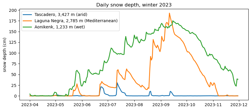
One winter (April–November 2023) in each climate zone: the arid Andes (Tascadero, CEAZA, 31° S), the Mediterranean Andes (Laguna Negra, DGA, 34° S) and the wet Andes of Patagonia (Aonikenk, IANIGLA, 49° S).

sites = {
    "450001": "Tascadero, 3,427 m (arid)",
    "5703009": "Laguna Negra, 2,785 m (Mediterranean)",
    "Aonikenk": "Aonikenk, 1,233 m (wet)",
}
winter_df = pd.DataFrame(
    client.get_data(list(sites), begin_date="2023-04-01", end_date="2023-11-30")
).assign(date=lambda df: pd.to_datetime(df["date"]))
print(winter_df["interval"].unique(), winter_df["units"].unique())
fig, ax = plt.subplots(figsize=(10, 4))
for sid, label in sites.items():
    site = winter_df[winter_df["station_id"] == sid]
    ax.plot(site["date"], site["value"], lw=2, label=label)
ax.set(ylabel="snow depth (cm)", title="Daily snow depth, winter 2023")
ax.legend()

<ArrowStringArray>
['daily']
Length: 1, dtype: str <ArrowStringArray>
['cm']
Length: 1, dtype: str

<matplotlib.legend.Legend object at 0x7fba82ac2850>

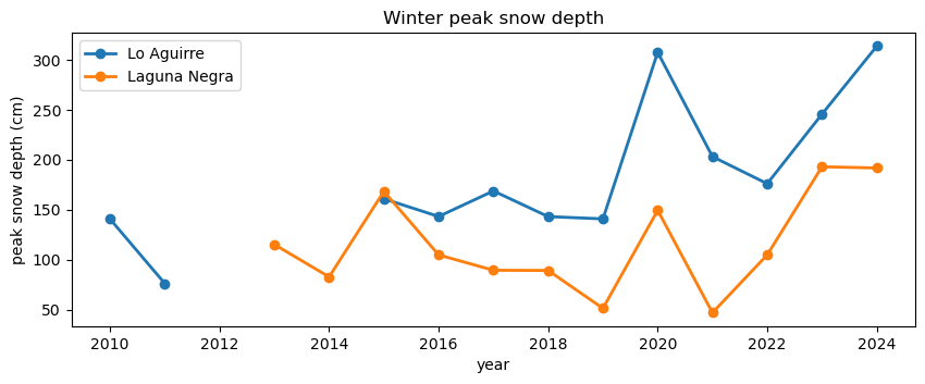
Winter peak depth at the two longest DGA records, Lo Aguirre (36° S, data from 2010) and Laguna Negra (34° S, from 2013). Years with less than half the April–October days observed are left out.

long_df = pd.DataFrame(client.get_data(["7301000", "5703009"])).assign(
    date=lambda df: pd.to_datetime(df["date"])
)
season = long_df[long_df["date"].dt.month.between(4, 10)]
peaks = season.groupby(["station_id", season["date"].dt.year])["value"].agg(
    ["max", "count"]
)
peaks = peaks[peaks["count"] >= 107]["max"].unstack("station_id")
print(peaks.round(1).to_string())
fig, ax = plt.subplots(figsize=(10, 3.5))
for sid, label in {"7301000": "Lo Aguirre", "5703009": "Laguna Negra"}.items():
    ax.plot(peaks.index, peaks[sid], marker="o", lw=2, label=label)
ax.set(xlabel="year", ylabel="peak snow depth (cm)", title="Winter peak snow depth")
ax.legend()

station_id  5703009  7301000
date
          NaN    140.6
          NaN     76.1
        115.1      NaN
         82.7      NaN
        168.3    160.9
        104.7    143.2
         89.3    168.7
         89.1    143.1
         51.2    140.8
        149.4    307.6
         46.8    203.1
        104.8    176.0
        193.0    245.7
        191.8    313.7

<matplotlib.legend.Legend object at 0x7fba6f947d90>