Sentinel-1 backscatter and the local incidence angle

Sentinel-1 RTC backscatter comes from Planetary Computer by default (10 m, 2014 onward, no account) with OPERA RTC-S1 as the 30 m burst-based alternative. The local incidence angle, which used to need a 350-line Earth Engine routine, now has a credential-free route: compute it from any DEM.

import matplotlib.pyplot as plt
import numpy as np

import easysnowdata as esd

aoi = (-121.94, 46.72, -121.54, 46.99)  # Mount Rainier

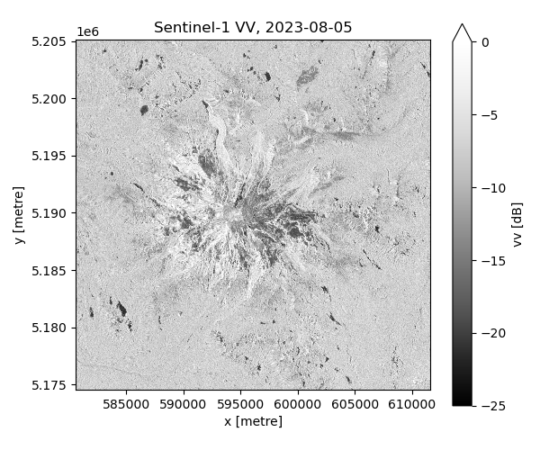
Two weeks of VV and VH backscatter, in dB, grouped one raster per pass.

s1 = esd.sar.sentinel1.load(
    aoi, "2023-08-01/2023-08-15", bands=["vv", "vh"], resolution=40
)
print(s1)

fig, ax = plt.subplots(figsize=(6, 5))
s1["vv"].isel(time=0).plot.imshow(ax=ax, cmap="Greys_r", vmin=-25, vmax=0)
ax.set_title(f"Sentinel-1 VV, {str(s1['time'].values[0])[:10]}")
ax.set_aspect("equal")
fig.tight_layout()

<xarray.Dataset> Size: 19MB
Dimensions:             (y: 764, x: 775, time: 4)
Coordinates:
  * y                   (y) float64 6kB 5.205e+06 5.205e+06 ... 5.175e+06
  * x                   (x) float64 6kB 5.806e+05 5.807e+05 ... 6.116e+05
  * time                (time) datetime64[us] 32B 2023-08-05T02:02:29.454706 ...
    sat:orbit_state     (time) object 32B 'ascending' ... 'descending'
    sat:relative_orbit  (time) int16 8B 137 13 64 115
    spatial_ref         int64 8B 0
Data variables:
    vv                  (time, y, x) float32 9MB dask.array<chunksize=(1, 764, 775), meta=np.ndarray>
    vh                  (time, y, x) float32 9MB dask.array<chunksize=(1, 764, 775), meta=np.ndarray>
Attributes:
    units:                 dB
    source:                planetary-computer
    source_id:             planetary-computer
    source_title:          Planetary Computer
    source_url:            https://planetarycomputer.microsoft.com/dataset/se...
    product_id:            sentinel-1-rtc
    title:                 Sentinel-1 radiometrically terrain-corrected backs...
    data_citation:         European Space Agency. Copernicus Sentinel-1 GRD. ...
    license:               Copernicus Sentinel data licence
    easysnowdata_version:  0.0.27.dev125+g480e638d6

The local incidence angle from the Copernicus DEM. No account, any orbit: the geometry differs between ascending and descending passes, which is why backscatter time series are usually split by relative orbit.

ascending = esd.sar.sentinel1.local_incidence_angle(
    aoi, source="dem", orbit_state="ascending", resolution=60
)
descending = esd.sar.sentinel1.local_incidence_angle(
    aoi, source="dem", orbit_state="descending", resolution=60
)

fig, axes = plt.subplots(1, 2, figsize=(11, 4.5), sharey=True)
for ax, ds, label in (
    (axes[0], ascending, "ascending"),
    (axes[1], descending, "descending"),
):
    ds["local_incidence_angle"].plot.imshow(ax=ax, cmap="magma", vmin=0, vmax=90)
    ax.set_title(f"Local incidence angle, {label}")
    ax.set_aspect("equal")
fig.tight_layout()

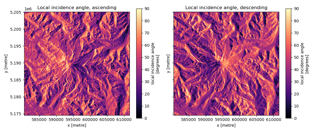
Where the two geometries disagree most is where terrain correction matters most: steep slopes that face one orbit and hide from the other.

difference = (
    ascending["local_incidence_angle"] - descending["local_incidence_angle"]
).compute()
print(f"max |ascending − descending|: {float(np.nanmax(np.abs(difference))):.1f}°")

max |ascending − descending|: 76.4°

With an Earthdata account, the OPERA static layers give the same angle as a published per-burst product, plus the layover and shadow mask:

opera = esd.sar.sentinel1.local_incidence_angle(aoi)      # source="opera-static"
esd.plotting.categorical(opera["mask"])                   # layover / shadow