Finnish snow courses (SYKE)

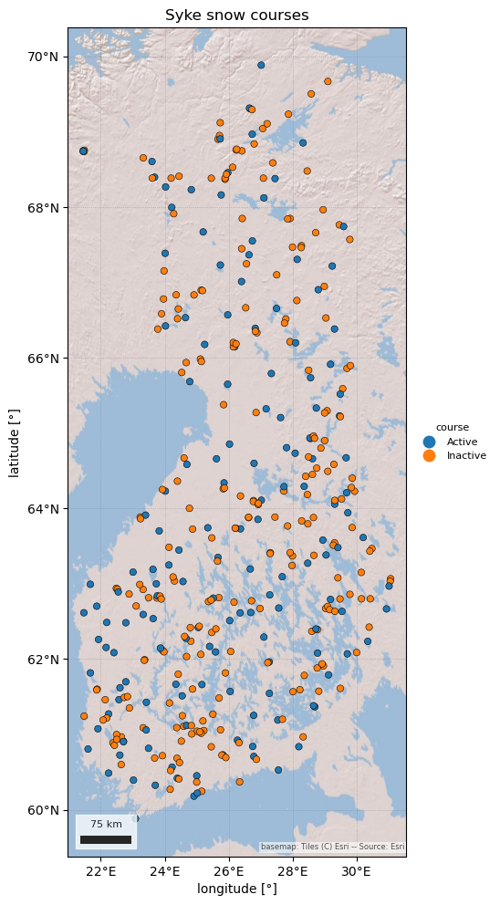
The Finnish Environment Institute (Syke) measures SWE along about 150 active snow courses, once a month from November to May, some since 1947. The open hydrology API (CC BY 4.0) serves the course SWE (no snow depth or density) and a derived areal SWE for drainage basins, twice a month.

SYKEClient reads the API, with no account. Every course record is "periodic". It is not part of esd.stations.inventory() or load().

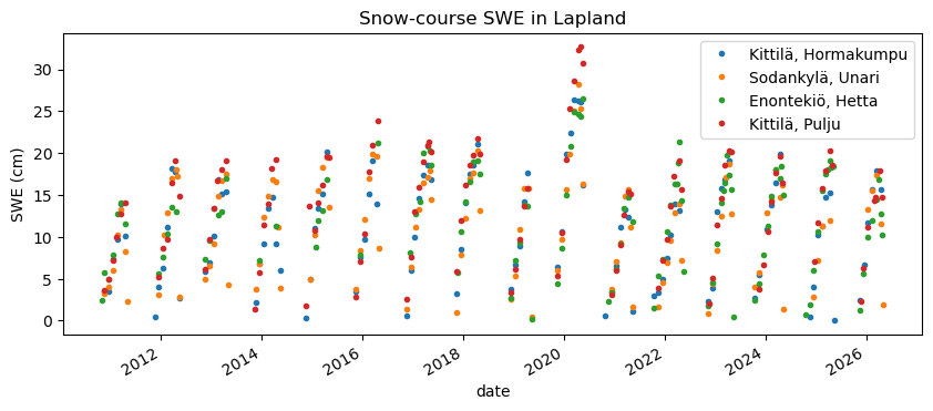
The figures show the active courses, and the monthly SWE at four Lapland courses since 2010.

import geopandas as gpd
import pandas as pd

import easysnowdata as esd
from easysnowdata.stations.clients import SYKEClient

client = SYKEClient()

Every snow course. status follows Syke’s own state: continuous courses are Active.

stations = client.get_all_stations()
stations_gdf = gpd.GeoDataFrame(
    pd.DataFrame(stations).set_index("station_id"),
    geometry=gpd.points_from_xy(
        [s["longitude"] for s in stations], [s["latitude"] for s in stations]
    ),
    crs="EPSG:4326",
)
print(stations_gdf["status"].value_counts().to_string())

ax = esd.plotting.points(
    stations_gdf, column="status", legend_label="course", title="Syke snow courses"
)

status
Inactive    242
Active      151
/home/runner/work/easysnowdata/easysnowdata/docs/gallery/station_datasets/plot_syke.py:38: GeographicAxesWarning: The data are in a geographic CRS (EPSG:4326), so one axis unit is a degree, not a metre. The axes use a latitude-corrected aspect (1/cos(64.9°) = 2.36) so shapes are not stretched; for a true equal-area grid load the product with crs='utm'.
  ax = esd.plotting.points(

Monthly SWE at four courses north of the Arctic Circle. Each point is one survey.

courses = ["1579", "1580", "1581", "1582"]
records = client.get_data(courses, begin_date="2010-09-01")
swe_df = (
    pd.DataFrame(records)
    .assign(date=lambda df: pd.to_datetime(df["date"]))
    .pivot_table(index="date", columns="station_id", values="value")
)
swe_df.columns = [stations_gdf.loc[c, "name"] for c in swe_df.columns]
ax = swe_df.plot(figsize=(10, 4), marker=".", linestyle="none")
ax.set(ylabel="SWE (cm)", title="Snow-course SWE in Lapland")

[Text(23.999999999999993, 0.5, 'SWE (cm)'), Text(0.5, 1.0, 'Snow-course SWE in Lapland')]

Areal SWE is a separate product: one value per drainage basin on the 1st and 16th of each month.

units = client.get_areal_units(active_only=True)
print(f"{len(units)} active areal-SWE units")

108 active areal-SWE units