Swiss long-term SWE (SLF)

The WSL Institute for Snow and Avalanche Research SLF has measured SWE by hand every two weeks at 11 sites between 1,200 and 2,540 m, some since 1936 (the GCOS SWE series). It also publishes daily snow depth from its manual study plots and its automated IMIS stations. Switzerland has no open daily SWE.

SLFClient(dataset=...) reads one dataset at a time: "gcos" (default, SWE every ~15 days), "new_snow" (2016–2022 new-snow SWE study), "study_plot" and "imis" (daily snow depth). Each uses its own station ids. Data are free with attribution to SLF (CC BY 4.0; GCOS: ODbL). It is not part of esd.stations.inventory() or load().

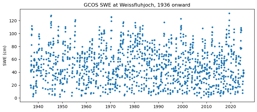
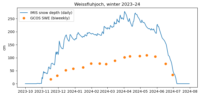
The figures show the GCOS SWE series at Weissfluhjoch since 1936, and one winter of IMIS daily snow depth next to the biweekly SWE.

import matplotlib.pyplot as plt
import pandas as pd

from easysnowdata.stations.clients import SLFClient

gcos = SLFClient(dataset="gcos")

The eleven GCOS sites.

sites_df = pd.DataFrame(gcos.get_all_stations()).set_index("station_id")
print(sites_df[["name", "elevation_m", "period_of_record"]].to_string())

                        name  elevation_m       period_of_record
station_id
1MR                   Mürren       1650.0  1949-02-01/2025-03-31
2AN                Andermatt       1440.0  1947-01-15/2025-03-31
2TR                  Trübsee       1780.0  1949-02-15/2025-04-15
4UL                 Ulrichen       1350.0  1950-12-15/2025-03-15
4ZE                  Zermatt       1600.0  1947-02-01/2025-02-15
5DF         Davos Flüelastr.       1560.0  1947-12-01/2025-03-20
5KK              Klosters KW       1200.0  1947-12-01/2025-03-03
5WJ            Weissfluhjoch       2540.0  1936-11-01/2025-05-31
6SB           San Bernardino       1640.0  1973-01-16/2025-04-11
7ST                Sta.Maria       1415.0  1968-02-08/2025-03-20
7ZU                     Zuoz       1710.0  1950-12-17/2025-03-14

Weissfluhjoch above Davos (2,540 m): every manual SWE measurement since 1936. Records are "periodic".

records = gcos.get_data("5WJ", variables="swe")
wfj_df = pd.DataFrame(records).assign(date=lambda df: pd.to_datetime(df["date"]))
print(wfj_df["interval"].unique(), len(wfj_df), "measurements")
fig, ax = plt.subplots(figsize=(10, 4))
ax.plot(wfj_df["date"], wfj_df["value"], ".")
ax.set(ylabel="SWE (cm)", title="GCOS SWE at Weissfluhjoch, 1936 onward")

<ArrowStringArray>
['periodic']
Length: 1, dtype: str 1384 measurements

[Text(23.999999999999993, 0.5, 'SWE (cm)'), Text(0.5, 1.0, 'GCOS SWE at Weissfluhjoch, 1936 onward')]

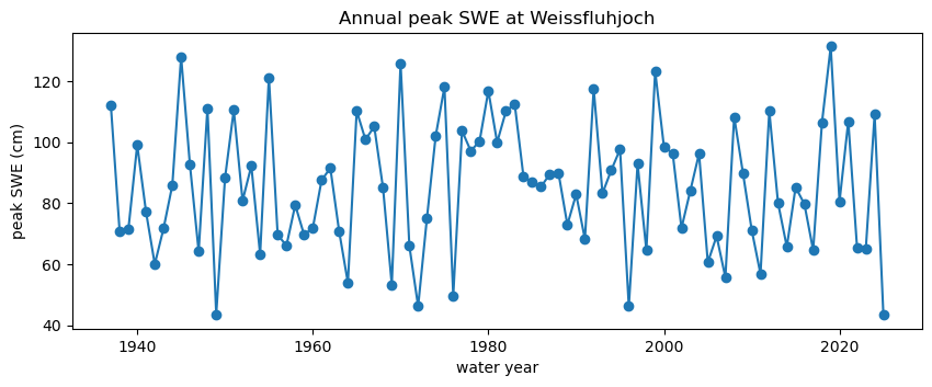
Peak SWE by water year shows the long-term record that only the manual series can give.

wfj_df["water_year"] = wfj_df["date"].dt.year + (wfj_df["date"].dt.month >= 10)
peak = wfj_df.groupby("water_year")["value"].max()
fig, ax = plt.subplots(figsize=(10, 3.5))
ax.plot(peak.index, peak.values, marker="o")
ax.set(
    xlabel="water year",
    ylabel="peak SWE (cm)",
    title="Annual peak SWE at Weissfluhjoch",
)

[Text(0.5, 24.0, 'water year'), Text(23.999999999999993, 0.5, 'peak SWE (cm)'), Text(0.5, 1.0, 'Annual peak SWE at Weissfluhjoch')]

The automated IMIS station at the same site (WFJ2) gives daily snow depth for the same winter as the biweekly SWE.

imis = SLFClient(dataset="imis")
depth_df = pd.DataFrame(
    imis.get_data(
        "WFJ2",
        variables="snwd",
        interval="daily",
        begin_date="2023-10-01",
        end_date="2024-07-31",
    )
).assign(date=lambda df: pd.to_datetime(df["date"]))
winter_df = wfj_df[(wfj_df["date"] >= "2023-10-01") & (wfj_df["date"] <= "2024-07-31")]
fig, ax = plt.subplots(figsize=(9, 4))
ax.plot(depth_df["date"], depth_df["value"], label="IMIS snow depth (daily)")
ax.plot(winter_df["date"], winter_df["value"], "o", label="GCOS SWE (biweekly)")
ax.set(ylabel="cm", title="Weissfluhjoch, winter 2023–24")
ax.legend()

<matplotlib.legend.Legend object at 0x7fba1042b9d0>