Automatic weather station examples

Eric Gagliano (egagli@uw.edu)
Updated: April 1st, 2024

Thanks for checking out these examples! The automatic_weather_station module is intended to make it easier to retrieve daily SNOTEL and CCSS data without having to do clunky downloads and conversions. Snow depth / SWE / PRCPSA are in meters, temperatures are in celsius. This module is built on my snotel_ccss_stations repository, which uses a github action to auto-update the station data daily.

%load_ext autoreload
%autoreload 2

%aimport easysnowdata

import pandas as pd
import geopandas as gpd
import numpy as np
import matplotlib.pyplot as plt
import datetime
import tqdm
import contextily as ctx

import xarray as xr
import glob

import requests 
from io import StringIO

View all SNOTEL & CCSS stations

• the SNOwpack TELemetry (SNOTEL) network includes over 800 automated weather stations in the Western U.S. for mountain snowpack observation

• the CCSS program manages a network of 130 automated snow sensors located in the Szierra Nevada and Shasta-Trinity Mountains

Get an up to date GeoDataFrame of all active SNOTEL and CCSS stations

# bbox_gdf = gpd.read_file('https://github.com/egagli/sar_snowmelt_timing/raw/main/input/shapefiles/mt_rainier.geojson')

StationCollection = easysnowdata.automatic_weather_stations.StationCollection()

Geodataframe with all stations has been added to the Station object. Please use the .all_stations attribute to access.
Use the .get_data(stations=geodataframe/string/list,variables=string/list,start_date=str,end_date=str) method to fetch data for specific stations and variables.

StationCollection.all_stations

	name	network	elevation_m	latitude	longitude	state	HUC	mgrs	mountainRange	beginDate	endDate	csvData	geometry
code
301_CA_SNTL	Adin Mtn	SNOTEL	1886.712036	41.235828	-120.791924	California	180200021403	10TFL	Great Basin Ranges	1983-10-01	2100-01-01	True	POINT (-120.79192 41.23583)
907_UT_SNTL	Agua Canyon	SNOTEL	2712.719971	37.522171	-112.271179	Utah	160300020301	12SUG	Colorado Plateau	1994-10-01	2100-01-01	True	POINT (-112.27118 37.52217)
916_MT_SNTL	Albro Lake	SNOTEL	2529.840088	45.597229	-111.959023	Montana	100200050701	12TVR	Central Montana Rocky Mountains	1996-09-01	2100-01-01	True	POINT (-111.95902 45.59723)
1267_AK_SNTL	Alexander Lake	SNOTEL	48.768002	61.749668	-150.889664	Alaska	190205051106	05VPJ	None	2014-08-28	2100-01-01	True	POINT (-150.88966 61.74967)
908_WA_SNTL	Alpine Meadows	SNOTEL	1066.800049	47.779572	-121.698471	Washington	171100100501	10TET	Cascade Range	1994-09-01	2100-01-01	True	POINT (-121.69847 47.77957)
...	...	...	...	...	...	...	...	...	...	...	...	...	...
SLT	Slate Creek	CCSS	1737.360000	41.043980	-122.480103	California	180200050304	10TEL	Klamath Mountains	2004-10-01	2024-04-02	True	POINT (-122.48010 41.04398)
SLI	Slide Canyon	CCSS	2804.160000	38.091234	-119.431881	California	180400090501	11SKC	Sierra Nevada	2005-10-01	2024-04-02	True	POINT (-119.43188 38.09123)
SLK	South Lake	CCSS	2926.080000	37.175903	-118.562660	California	180901020601	11SLB	Sierra Nevada	2004-10-01	2024-04-02	True	POINT (-118.56266 37.17590)
STL	State Lakes	CCSS	3169.920000	36.926483	-118.573250	California	180300100305	11SLA	Sierra Nevada	2018-11-01	2024-04-02	True	POINT (-118.57325 36.92648)
TMR	Tamarack Summit	CCSS	2301.240000	37.163750	-119.200531	California	180400060903	11SLB	Sierra Nevada	2011-01-01	2024-04-02	True	POINT (-119.20053 37.16375)

969 rows × 13 columns

Use geopandas GeoDataFrame.explore() on the all_stations geodataframe to interactively view the stations

• color by network: red is SNOTEL, blue is CCSS.

StationCollection.all_stations.astype(dict(beginDate=str, endDate=str)).explore(
    column="network", cmap="bwr"
)

Make this Notebook Trusted to load map: File -> Trust Notebook

Get data for a singular site: Is our winter on track with the historical record at the Paradise, WA SNOTEL station?

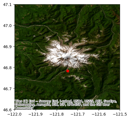
• check out information about the SNOTEL station near Mt. Rainier at Paradise, WA

• cool plots available at the Northwest River Forecast Center website

Select a station code (which you can find in this interactive plot, or by other means)

• for SNOTEL stations, this will be of the form {unique number}_{two letter state abbreviation}_SNTL (e.g. 679_WA_SNTL).

• for CCSS stations, this will be a three letter code (e.g. BLK).

ParadiseSNOTEL = easysnowdata.automatic_weather_stations.StationCollection()

Geodataframe with all stations has been added to the Station object. Please use the .all_stations attribute to access.
Use the .get_data(stations=geodataframe/string/list,variables=string/list,start_date=str,end_date=str) method to fetch data for specific stations and variables.

ParadiseSNOTEL.get_data("679_WA_SNTL")

Only one station chosen with variables=None. Default behavior fetches all variables for this station.
Dataframe has been added to the Station object. Please use the .data attribute to access.

f, ax = plt.subplots()

ParadiseSNOTEL.stations.plot(ax=ax, color="red")

ax.set_xlim(-122, -121.5)
ax.set_ylim(46.6, 47.1)

ctx.add_basemap(
    ax, crs=ParadiseSNOTEL.stations.crs, source=ctx.providers.Esri.WorldImagery
)

ParadiseSNOTEL.data

	TAVG	TMIN	TMAX	SNWD	WTEQ	PRCPSA
datetime
1980-10-01	NaN	NaN	NaN	NaN	0.0000	0.0000
1980-10-02	NaN	NaN	NaN	NaN	0.0000	0.0000
1980-10-03	NaN	NaN	NaN	NaN	0.0000	0.0000
1980-10-04	NaN	NaN	NaN	NaN	0.0000	0.0000
1980-10-05	NaN	NaN	NaN	NaN	0.0000	0.0000
...	...	...	...	...	...	...
2024-03-28	-1.0	-2.2	1.9	3.0480	1.4376	0.0102
2024-03-29	0.2	-3.5	5.7	3.1750	1.4478	0.0000
2024-03-30	1.5	-3.2	8.3	3.1242	1.4478	0.0025
2024-03-31	1.1	-3.4	6.9	3.1242	1.4503	0.0000
2024-04-01	NaN	NaN	NaN	3.0734	1.4453	NaN

15889 rows × 6 columns

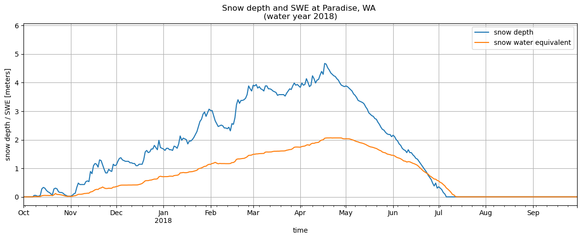
Try a simple plot of snow depth and SWE

• select the column of interest and use pandas built in Series.plot()

f, ax = plt.subplots(figsize=(12, 5))

ParadiseSNOTEL.data["SNWD"].plot(ax=ax, label="snow depth")
ParadiseSNOTEL.data["WTEQ"].plot(ax=ax, label="snow water equivalent")

ax.set_xlim(pd.to_datetime(["2017-10-01", "2018-09-30"]))

ax.grid()
ax.legend()

ax.set_xlabel("time")
ax.set_ylabel("snow depth / SWE [meters]")
ax.set_title("Snow depth and SWE at Paradise, WA \n(water year 2018)")

f.tight_layout()

Try a more complex plot that shows current snow depth against statistics calculated from the entire time series for each day of water year

• water year is conceptual 12 month period used to describe when the bulk of precipitation falls, mostly used for hydrology attribution

  • in the northern hemisphere, we usually define the water year to start October 1st and go until September 30th (e.g. water year 2017: October 1st, 2016 - September 30th, 2017)

  • so October 1st is DOWY 1

• try a function like easysnowdata.utils.datetime_to_DOWY() to convert datetimes to day of water year and add a dedicated DOWY column

  • this function should account for leap years

• then use pandas groupby functionality to calculate stats per DOWY

• plot these stats

  • thanks David Shean for the plot inspiration!

ParadiseSNOTEL.data["DOWY"] = ParadiseSNOTEL.data.index.map(
    easysnowdata.utils.datetime_to_DOWY
)
ParadiseSNOTEL.data["WY"] = ParadiseSNOTEL.data.index.map(
    easysnowdata.utils.datetime_to_WY
)

ParadiseSNOTEL.data

	TAVG	TMIN	TMAX	SNWD	WTEQ	PRCPSA	DOWY	WY
datetime
1980-10-01	NaN	NaN	NaN	NaN	0.0000	0.0000	1	1981
1980-10-02	NaN	NaN	NaN	NaN	0.0000	0.0000	2	1981
1980-10-03	NaN	NaN	NaN	NaN	0.0000	0.0000	3	1981
1980-10-04	NaN	NaN	NaN	NaN	0.0000	0.0000	4	1981
1980-10-05	NaN	NaN	NaN	NaN	0.0000	0.0000	5	1981
...	...	...	...	...	...	...	...	...
2024-03-28	-1.0	-2.2	1.9	3.0480	1.4376	0.0102	180	2024
2024-03-29	0.2	-3.5	5.7	3.1750	1.4478	0.0000	181	2024
2024-03-30	1.5	-3.2	8.3	3.1242	1.4478	0.0025	182	2024
2024-03-31	1.1	-3.4	6.9	3.1242	1.4503	0.0000	183	2024
2024-04-01	NaN	NaN	NaN	3.0734	1.4453	NaN	184	2024

15889 rows × 8 columns

stat_list = ["min", "max", "mean", "std", "median"]
paradise_snotel_DOWY_snwd_stats = ParadiseSNOTEL.data.groupby("DOWY").agg(stat_list)[
    "SNWD"
]
paradise_snotel_DOWY_snwd_stats

	min	max	mean	std	median
DOWY
1	0.0	0.2286	0.014111	0.053862	0.0
2	0.0	0.2032	0.011289	0.047895	0.0
3	0.0	0.2286	0.014111	0.053862	0.0
4	0.0	0.1270	0.012700	0.032888	0.0
5	0.0	0.1270	0.012700	0.034022	0.0
...	...	...	...	...	...
362	0.0	0.0254	0.001411	0.005987	0.0
363	0.0	0.0254	0.001411	0.005987	0.0
364	0.0	0.0254	0.002822	0.008214	0.0
365	0.0	0.0762	0.005644	0.018595	0.0
366	0.0	0.0000	0.000000	0.000000	0.0

366 rows × 5 columns

today = datetime.datetime.today().strftime("%Y-%m-%d")
current_WY = slice(f"{int(today[0:4])-1}-10-01", f"{today}")
current_WY_paradise_snotel = ParadiseSNOTEL.data[current_WY.start : current_WY.stop]

f, ax = plt.subplots(figsize=(12, 7))

for stat, stat_color in zip(
    ["min", "max", "mean", "median"], ["red", "blue", "mediumpurple", "mediumseagreen"]
):
    ax.plot(
        paradise_snotel_DOWY_snwd_stats.index,
        paradise_snotel_DOWY_snwd_stats[stat],
        label=stat,
        color=stat_color,
        linewidth=3,
    )

ax.fill_between(
    paradise_snotel_DOWY_snwd_stats.index,
    paradise_snotel_DOWY_snwd_stats["mean"] - paradise_snotel_DOWY_snwd_stats["std"],
    paradise_snotel_DOWY_snwd_stats["mean"] + paradise_snotel_DOWY_snwd_stats["std"],
    color="mediumpurple",
    alpha=0.3,
    label="mean +/- 1 std",
)

ax.scatter(
    current_WY_paradise_snotel.DOWY,
    current_WY_paradise_snotel.SNWD,
    marker="o",
    color="black",
    label="Current WY",
)

ax.set_xlim([0, 366])
ax.set_ylim([0, 6])

ax.grid()
ax.legend()

ax.set_title(
    f"Current snow depth against historical snow depth stats by DOWY at Paradise, WA\n({ParadiseSNOTEL.data.index.min().date()} - {ParadiseSNOTEL.data.index.max().date()})"
)
ax.set_xlabel("Day of Water Year [Oct 1 - Sept 30]")
ax.set_ylabel("Snow depth [meters]")
f.tight_layout()

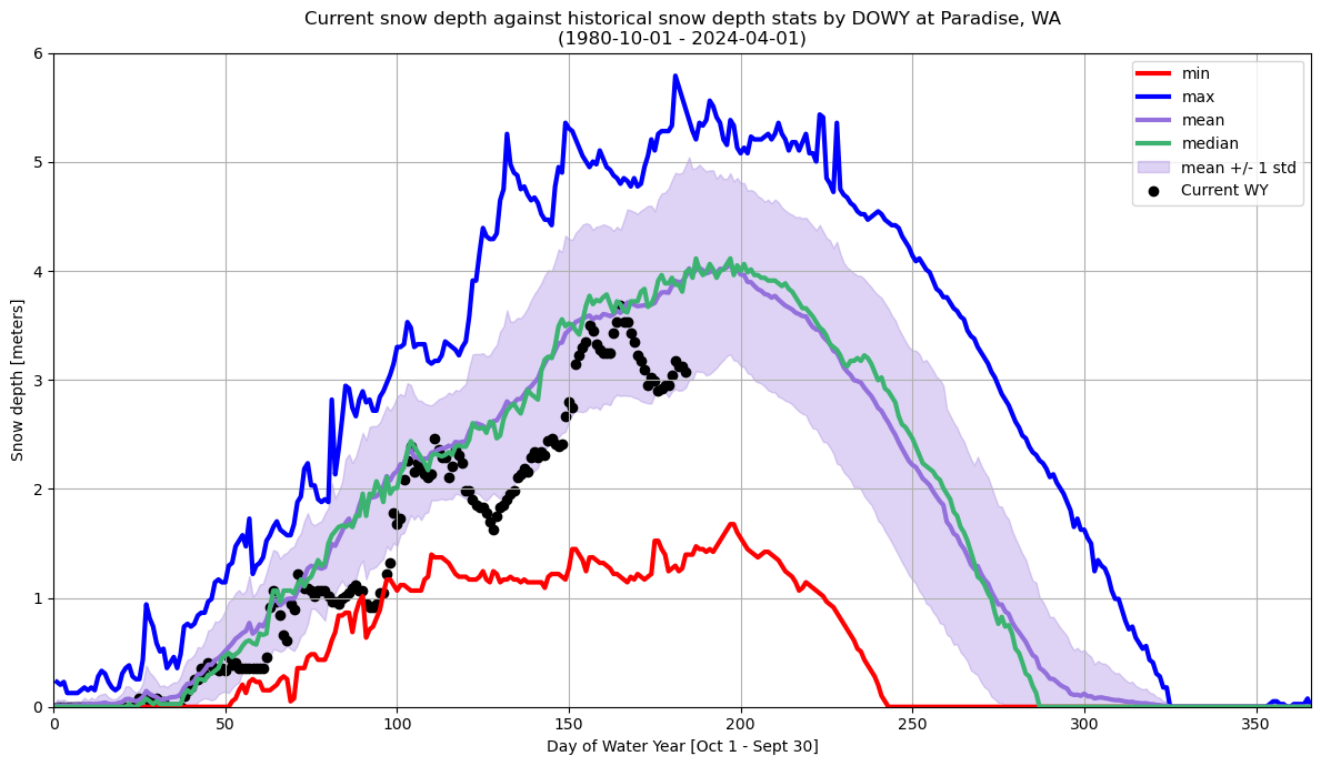
Looks like we’re slightly below the mean for snow depth for today’s DOWY.

Read a variable from a list of stations: Does the SNOTEL network and CCSS network list the same station?

• no controversy here, but i noticed that a station name was repeated

• perhaps both networks have data from the same station accessible

• might make sense if they are co-managed in some way?

Create a list of the stations we are interested in and pass it in to our get_data() function

station_list = ["356_CA_SNTL", "BLK"]

TwoStations = easysnowdata.automatic_weather_stations.StationCollection()

Geodataframe with all stations has been added to the Station object. Please use the .all_stations attribute to access.
Use the .get_data(stations=geodataframe/string/list,variables=string/list,start_date=str,end_date=str) method to fetch data for specific stations and variables.

TwoStations.get_data(station_list, variables="WTEQ")

WTEQ dataframe has been added to the Station object. Please use the .WTEQ attribute to access the dataframe.
Full ['WTEQ'] dataset has been added to the station object. Please use the .data attribute to access the dataset.

100%|██████████| 2/2 [00:00<00:00,  2.31it/s]

TwoStations.WTEQ

	356_CA_SNTL	BLK
datetime
1980-07-09	NaN	NaN
1980-07-10	NaN	NaN
1980-07-11	NaN	NaN
1980-07-12	NaN	NaN
1980-07-13	NaN	NaN
...	...	...
2024-03-29	0.8204	0.8204
2024-03-30	0.8433	0.8433
2024-03-31	0.8484	0.8484
2024-04-01	0.8534	0.8534
2024-04-02	NaN	0.8534

15974 rows × 2 columns

Plot the two stations on the same axis

• if we properly set the index as the datetime, and we used parse_dates=True, these should line up!

f, ax = plt.subplots(figsize=(20, 7))

TwoStations.WTEQ.plot(ax=ax, color=["red", "blue"])

ax.legend()

ax.set_xlabel("time")
ax.set_ylabel("snow water equivalent [meters]")
ax.set_title("SNOTEL and CCSS SWE at Blue Lakes, CA \nmaybe these are the same? :)")

f.tight_layout()

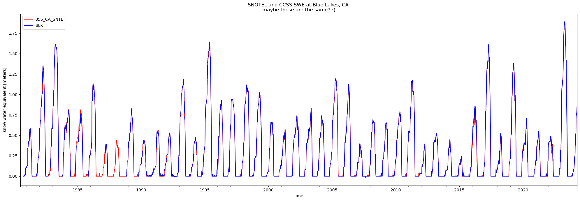
These look oddly similar… let’s check out their correlation

• convenient built in DataFrame.corr()

TwoStations.WTEQ.corr()

	356_CA_SNTL	BLK
356_CA_SNTL	1.000000	0.999056
BLK	0.999056	1.000000

These correlation values, along with the time series above, makes me think these are way too similar… no way these would agree this much even if the stations were right next to each other!

Let’s see where they exist spatially

• select the stations by index and reproject to UTM 11N

• use contextily for a basemap

TwoStations.stations

	name	network	elevation_m	latitude	longitude	state	HUC	mgrs	mountainRange	beginDate	endDate	csvData	geometry
code
356_CA_SNTL	Blue Lakes	SNOTEL	2458.821533	38.608002	-119.92437	California	180400120101	11SKC	Sierra Nevada	1980-10-01	2100-01-01	True	POINT (-119.92437 38.60800)
BLK	Blue Lakes	CCSS	2438.400000	38.613000	-119.93100	California	180400120101	11SKC	Sierra Nevada	2004-10-01	2024-04-02	True	POINT (-119.93100 38.61300)

f, ax = plt.subplots(figsize=(7, 7))


TwoStations.stations.to_crs("EPSG:32611").loc[['356_CA_SNTL']].plot(ax=ax, color='red',label='356_CA_SNTL')
TwoStations.stations.to_crs("EPSG:32611").loc[['BLK']].plot(ax=ax, color='blue',label='BLK')


ax.set_xlim([244200, 245700])
ax.set_ylim([4276900, 4278700])

ctx.add_basemap(ax, crs="EPSG:32611", source=ctx.providers.Esri.WorldImagery)

ax.legend() # add labels here

f.tight_layout()

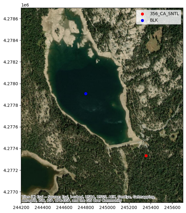
Interesting locations :) Based on correlation and location, I’m going to say these are the same! Wonder what those tiny differences are about…

Look’s like some of the CCSS stations have “Natural Resources Conservation Service” as their operator

• Let’s check which stations these are!

• Let’s plot these shared stations in red, and not shared in blue

csv = 'https://cdec.water.ca.gov/misc/SnowSensors.html'
response = requests.get(csv)
same_stations_df = pd.read_html(StringIO(response.content.decode('utf-8')))[0].set_index('ID').sort_index()
same_stations_df = same_stations_df[same_stations_df.nunique(axis=1) > 1]
same_stations_gdf = gpd.GeoDataFrame(same_stations_df, geometry=gpd.points_from_xy(same_stations_df['Longitude'], same_stations_df['Latitude']))
same_stations_gdf.crs = "EPSG:4326"
same_stations_gdf = same_stations_gdf[same_stations_gdf['Operator Agency']=='Natural Resources Conservation Service']
same_stations_gdf

	Name	Elev (feet)	Latitude	Longitude	April 1 Avg (inches)	Operator Agency	geometry
ID
ADM	ADIN MOUNTAIN	6200	41.237	-120.792	13.6	Natural Resources Conservation Service	POINT (-120.79200 41.23700)
BLK	BLUE LAKES	8000	38.613	-119.931	33.1	Natural Resources Conservation Service	POINT (-119.93100 38.61300)
BMW	BIG MEADOWS (SCS)	8700	39.458	-119.946	25.7	Natural Resources Conservation Service	POINT (-119.94600 39.45800)
BSK	BURNSIDE LAKE	8129	38.719	-119.894	-9999.0	Natural Resources Conservation Service	POINT (-119.89400 38.71900)
CDP	CEDAR PASS	7100	41.583	-120.303	18.1	Natural Resources Conservation Service	POINT (-120.30300 41.58300)
CSL	CENT SIERRA SNOW LAB	6900	39.325	-120.367	33.6	Natural Resources Conservation Service	POINT (-120.36700 39.32500)
CWF	CROWDER FLAT	5100	41.893	-120.752	-9999.0	Natural Resources Conservation Service	POINT (-120.75200 41.89300)
CXS	CARSON PASS	8353	38.692	-120.002	-9999.0	Natural Resources Conservation Service	POINT (-120.00200 38.69200)
DSS	DISMAL SWAMP	7050	41.993	-120.165	29.2	Natural Resources Conservation Service	POINT (-120.16500 41.99300)
EBB	EBBETTS PASS	8700	38.561	-119.808	38.8	Natural Resources Conservation Service	POINT (-119.80800 38.56100)
EP5	ECHO PEAK 5	7800	38.849	-120.079	39.5	Natural Resources Conservation Service	POINT (-120.07900 38.84900)
FLL	FALLEN LEAF LAKE	6250	38.932	-120.056	7.0	Natural Resources Conservation Service	POINT (-120.05600 38.93200)
HGM	HAGANS MEADOW	8000	38.853	-119.940	16.5	Natural Resources Conservation Service	POINT (-119.94000 38.85300)
HVN	HEAVENLY VALLEY	8800	38.929	-119.917	28.1	Natural Resources Conservation Service	POINT (-119.91700 38.92900)
IDC	INDEPENDENCE CAMP	7000	39.453	-120.299	21.8	Natural Resources Conservation Service	POINT (-120.29900 39.45300)
IDP	INDEPENDENCE LAKE (SCS)	8450	39.435	-120.322	41.4	Natural Resources Conservation Service	POINT (-120.32200 39.43500)
INN	INDEPENDENCE CREEK	6500	39.494	-120.293	12.7	Natural Resources Conservation Service	POINT (-120.29300 39.49400)
LBD	LOBDELL LAKE	9200	38.440	-119.377	17.3	Natural Resources Conservation Service	POINT (-119.37700 38.44000)
LVM	LEAVITT MEADOWS	7200	38.305	-119.552	8.0	Natural Resources Conservation Service	POINT (-119.55200 38.30500)
LVT	LEAVITT LAKE	9600	38.282	-119.621	-9999.0	Natural Resources Conservation Service	POINT (-119.62100 38.28200)
MNT	MONITOR PASS	8350	38.670	-119.615	-9999.0	Natural Resources Conservation Service	POINT (-119.61500 38.67000)
MRL	MARLETTE LAKE	8000	39.173	-119.905	21.1	Natural Resources Conservation Service	POINT (-119.90500 39.17300)
MSK	MOUNT ROSE SKI AREA	8900	39.326	-119.902	38.5	Natural Resources Conservation Service	POINT (-119.90200 39.32600)
PSN	POISON FLAT	7900	38.501	-119.631	16.2	Natural Resources Conservation Service	POINT (-119.63100 38.50100)
RP2	RUBICON PEAK 2	7500	39.001	-120.140	29.1	Natural Resources Conservation Service	POINT (-120.14000 39.00100)
SDW	SUMMIT MEADOW	9313	38.398	-119.536	-9999.0	Natural Resources Conservation Service	POINT (-119.53600 38.39800)
SPS	SONORA PASS BRIDGE	8750	38.318	-119.601	26.0	Natural Resources Conservation Service	POINT (-119.60100 38.31800)
SPT	SPRATT CREEK	6150	38.666	-119.817	4.5	Natural Resources Conservation Service	POINT (-119.81700 38.66600)
SQV	SQUAW VALLEY GOLD COAST	8200	39.194	-120.276	46.5	Natural Resources Conservation Service	POINT (-120.27600 39.19400)
TCC	TAHOE CITY CROSS	6750	39.171	-120.155	16.0	Natural Resources Conservation Service	POINT (-120.15500 39.17100)
TK2	TRUCKEE 2	6400	39.300	-120.194	14.3	Natural Resources Conservation Service	POINT (-120.19400 39.30000)
VRG	VIRGINIA LAKES RIDGE	9300	38.077	-119.234	20.3	Natural Resources Conservation Service	POINT (-119.23400 38.07700)
WC3	WARD CREEK 3	6750	39.136	-120.219	39.4	Natural Resources Conservation Service	POINT (-120.21900 39.13600)

f, ax = plt.subplots(figsize=(10, 10))

same_stations_gdf.to_crs("EPSG:32611").plot(
    ax=ax, color="red", label="CCSS station operated by NRCS"
)
ccss_stations_gdf = TwoStations.all_stations[
    TwoStations.all_stations["network"] == "CCSS"
].to_crs("EPSG:32611")
ccss_stations_gdf[~ccss_stations_gdf.index.isin(same_stations_gdf.index)].plot(
    ax=ax, color="blue", label="CCSS station not operated by NRCS"
)

ctx.add_basemap(ax, crs="EPSG:32611", source=ctx.providers.Esri.WorldImagery)

ax.legend()

f.tight_layout()

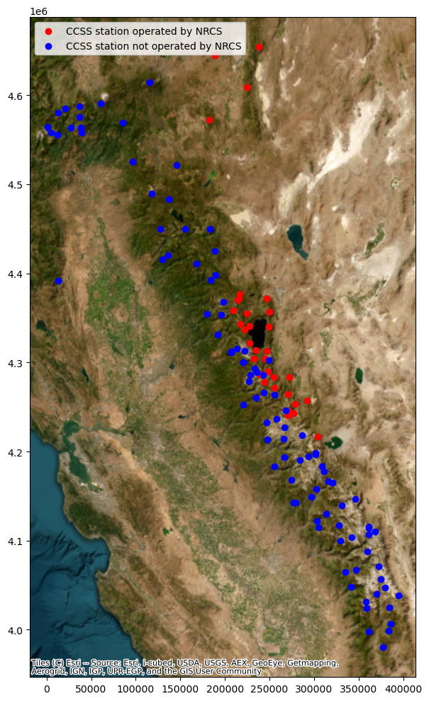
There are 33 of these! These are likely also listed as SNOTEL stations…

Read a variable using a geodataframe: How extraordinary was the California 2023 snowpack?

• the Sierra Nevada received a historic amount of snow in 2023

• let’s explore the magnitude of this season by comparing to the median snow pack

Let’s bring in only CCSS stations

• Filter the all_stations geodataframe with network == CCSS, and pass the filtered geodatframe to the get_data() function.

ccssStations = easysnowdata.automatic_weather_stations.StationCollection()

Geodataframe with all stations has been added to the Station object. Please use the .all_stations attribute to access.
Use the .get_data(stations=geodataframe/string/list,variables=string/list,start_date=str,end_date=str) method to fetch data for specific stations and variables.

ccss_only = ccssStations.all_stations[ccssStations.all_stations.network == "CCSS"]

ccssStations.get_data(stations=ccss_only,variables="WTEQ")

WTEQ dataframe has been added to the Station object. Please use the .WTEQ attribute to access the dataframe.
Full ['WTEQ'] dataset has been added to the station object. Please use the .data attribute to access the dataset.

  0%|          | 0/130 [00:00<?, ?it/s]
100%|██████████| 130/130 [00:41<00:00,  3.17it/s]

Let’s check out the percent of normal snow depth for April 1st, 2023

• let’s add a DOWY column to the ccssStations.WTEQ dataframe like before, groupby DOWY, apply a median, and divide the observation on April 1st, 2023 by the DOWY 183 (April 1) median

  • add these percent normal values back to ccssStations.stations

• will need to do some slight cleaning to get rid of NaNs, Infs, physically impossible values…

ccssStations.WTEQ["DOWY"] = ccssStations.WTEQ.index.map(
    easysnowdata.utils.datetime_to_DOWY
)
ccssStations.WTEQ["WY"] = ccssStations.WTEQ.index.map(easysnowdata.utils.datetime_to_WY)

ccssStations.stations.loc[:, "april2023_percent_norm"] = 100 * (
    ccssStations.WTEQ["2023-04-01":"2023-04-01"].squeeze()
    / ccssStations.WTEQ.groupby("DOWY").median().loc[183]
)

/home/eric/miniconda3/envs/easysnowdata/lib/python3.12/site-packages/geopandas/geodataframe.py:1525: SettingWithCopyWarning: 
A value is trying to be set on a copy of a slice from a DataFrame.
Try using .loc[row_indexer,col_indexer] = value instead

See the caveats in the documentation: https://pandas.pydata.org/pandas-docs/stable/user_guide/indexing.html#returning-a-view-versus-a-copy
  super().__setitem__(key, value)

ccssStations.stations = ccssStations.stations.dropna(subset="april2023_percent_norm")
ccssStations.stations = ccssStations.stations[
    ccssStations.stations["april2023_percent_norm"] < 7500
]

View the values in order…

• use .sort_values() function to get an idea of percent normal snow depth values

• DataFrame.head() and DataFrame.tail() to see highest and lowest percent normal snow depth values

ccssStations.stations.sort_values("april2023_percent_norm", ascending=False).head()

	name	network	elevation_m	latitude	longitude	state	HUC	mgrs	mountainRange	beginDate	endDate	csvData	geometry	april2023_percent_norm
code
BCH	Beach Meadows	CCSS	2331.7200	36.126095	-118.293457	California	180300010403	11SLV	Sierra Nevada	2004-10-01	2024-04-03	True	POINT (-118.29346 36.12609)	7365.789474
FLL	Fallen Leaf Lake	CCSS	1905.0000	38.932000	-120.056000	California	160501010401	10SGJ	None	2004-10-01	2024-04-03	True	POINT (-120.05600 38.93200)	4525.764192
LVM	Leavitt Meadows	CCSS	2194.5600	38.305000	-119.552000	California	160503020104	11SKC	Sierra Nevada	2004-10-01	2024-04-03	True	POINT (-119.55200 38.30500)	706.728704
GNF	Giant Forest (Usace)	CCSS	1950.7200	36.562867	-118.770283	California	180300070402	11SLA	Sierra Nevada	NaT	2024-04-03	True	POINT (-118.77028 36.56287)	700.401606
DPO	Devils Postpile	CCSS	2307.0312	37.629410	-119.084671	California	180400060402	11SLB	Sierra Nevada	2007-10-01	2024-04-03	True	POINT (-119.08467 37.62941)	642.842557

ccssStations.stations.sort_values("april2023_percent_norm", ascending=False).tail()

	name	network	elevation_m	latitude	longitude	state	HUC	mgrs	mountainRange	beginDate	endDate	csvData	geometry	april2023_percent_norm
code
CDP	Cedar Pass	CCSS	2164.0800	41.583000	-120.303000	California	180200020603	10TGM	Great Basin Ranges	NaT	2024-04-03	True	POINT (-120.30300 41.58300)	165.316340
SQV	Palisades Tahoe Snotel	CCSS	2499.3600	39.194000	-120.276000	California	160501020202	10SGJ	Sierra Nevada	2004-10-01	2024-04-03	True	POINT (-120.27600 39.19400)	165.202219
DSS	Dismal Swamp	CCSS	2148.8400	41.993000	-120.165000	California	171200070304	10TGM	Great Basin Ranges	NaT	2024-04-03	True	POINT (-120.16500 41.99300)	148.136711
LLP	Lower Lassen Peak	CCSS	2541.4224	40.466602	-121.508110	California	180201560301	10TFK	Cascade Range	2004-10-01	2024-04-03	True	POINT (-121.50811 40.46660)	146.590403
SHM	Shimmy Lake	CCSS	1950.7200	41.005299	-122.801598	California	180102110501	10TEL	Klamath Mountains	2005-10-01	2024-01-23	True	POINT (-122.80160 41.00530)	123.362639

Plot the percent of normal snow depths for April 1st, 2023

• add elevation plot to the right with horizontal dashed line at 100% (normal)

f, ax = plt.subplots(1, 2, figsize=(12, 9), gridspec_kw={"width_ratios": [2, 1]})

ccssStations.stations.to_crs("EPSG:32611").plot(
    ax=ax[0],
    column="april2023_percent_norm",
    legend=True,
    vmin=0,
    vmax=500,
    cmap="gnuplot",
    edgecolor="black",
    s=100,
)

ctx.add_basemap(
    ax[0], crs="EPSG:32611", source=ctx.providers.Esri.WorldImagery, attribution=""
)

ax[0].set_title("station locations")


ax[1].scatter(
    ccssStations.stations.elevation_m,
    ccssStations.stations.april2023_percent_norm,
    c=ccssStations.stations.april2023_percent_norm,
    cmap="gnuplot",
    vmin=0,
    vmax=500,
    edgecolors="black",
    s=100,
)
ax[1].axhline(y=100, linestyle="--", color="black")

ax[1].set_title("station percent normal snow depth vs elevation")
ax[1].set_xlabel("elevation [m]")
ax[1].set_ylabel("percent of normal snow depth [%]")

ax[1].set_ylim([0, 1000])

f.suptitle(f"California percent normal snow depth for April 1st, 2023")
f.tight_layout()

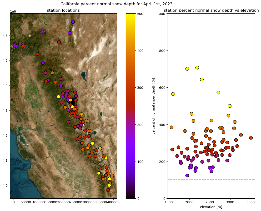
Looks like a lot more snow than usual to me!

Read a variable from all CSVs by looping over the entire geodataframe: Has the date of maximum SWE changed in the Western US?

• Snowmelt timing can be an important indicator of regional climate change, and the snowmelt timing of the Western U.S. is projected to shift earlier in the year by up to 1 month by 2050 (Barnett et al., 2005; Stewart, 2009), with a corresponding snowpack loss equivalent to a 25% decrease in streamflow from snowmelt (Siirila-Woodburn et al., 2021).

• Let’s explore trends in maximum SWE timing using SNOTEL and CCSS stations

This time we will get SWE at every station

• might take a minute to load in almost 1000 CSVs…

• store SWE for all stations in all_stations_swe_df

%%time 

WesternUS = easysnowdata.automatic_weather_stations.StationCollection()
WesternUS.get_data(WesternUS.all_stations,variables="WTEQ")

Geodataframe with all stations has been added to the Station object. Please use the .all_stations attribute to access.
Use the .get_data(stations=geodataframe/string/list,variables=string/list,start_date=str,end_date=str) method to fetch data for specific stations and variables.
WTEQ dataframe has been added to the Station object. Please use the .WTEQ attribute to access the dataframe.
Full ['WTEQ'] dataset has been added to the station object. Please use the .data attribute to access the dataset.
CPU times: user 14.4 s, sys: 1.24 s, total: 15.6 s
Wall time: 9min 44s

100%|██████████| 969/969 [09:40<00:00,  1.67it/s]

all_stations_swe_df = WesternUS.WTEQ
all_stations_swe_df

	301_CA_SNTL	907_UT_SNTL	916_MT_SNTL	1267_AK_SNTL	908_WA_SNTL	1189_AK_SNTL	1062_AK_SNTL	1070_AK_SNTL	302_OR_SNTL	1000_OR_SNTL	...	QUA	LLP	FOR	GEM	WTM	SLT	SLI	SLK	STL	TMR
datetime
1909-04-13	NaN	NaN	NaN	NaN	NaN	NaN	NaN	NaN	NaN	NaN	...	NaN	NaN	NaN	NaN	NaN	NaN	NaN	NaN	NaN	NaN
1954-12-01	NaN	NaN	NaN	NaN	NaN	NaN	NaN	NaN	NaN	NaN	...	NaN	NaN	NaN	NaN	NaN	NaN	NaN	NaN	0.0635	NaN
1954-12-02	NaN	NaN	NaN	NaN	NaN	NaN	NaN	NaN	NaN	NaN	...	NaN	NaN	NaN	NaN	NaN	NaN	NaN	NaN	0.0635	NaN
1954-12-03	NaN	NaN	NaN	NaN	NaN	NaN	NaN	NaN	NaN	NaN	...	NaN	NaN	NaN	NaN	NaN	NaN	NaN	NaN	0.0635	NaN
1954-12-04	NaN	NaN	NaN	NaN	NaN	NaN	NaN	NaN	NaN	NaN	...	NaN	NaN	NaN	NaN	NaN	NaN	NaN	NaN	0.1143	NaN
...	...	...	...	...	...	...	...	...	...	...	...	...	...	...	...	...	...	...	...	...	...
2024-03-29	0.4267	0.2896	0.3175	0.2464	0.8839	0.1448	0.3251	0.3327	0.3937	1.1354	...	NaN	2.4755	0.4846	NaN	0.5893	1.0119	0.8110	0.3155	0.6106	0.7503
2024-03-30	0.4318	0.2896	0.3175	0.2489	0.8865	0.1448	0.3251	0.3378	0.3962	1.1379	...	NaN	2.5098	0.4953	NaN	0.6017	1.0363	0.8364	0.3338	0.6243	0.7777
2024-03-31	0.4318	0.2972	0.3200	0.2692	0.8865	0.1448	0.3327	0.3454	0.3988	1.1379	...	NaN	2.5240	0.5080	NaN	0.6078	1.0516	0.8407	0.3399	0.6314	0.7930
2024-04-01	0.4191	0.3048	0.3353	0.2692	0.8839	0.1448	0.3378	0.3556	0.3962	1.1328	...	NaN	2.5250	0.5182	NaN	0.6081	1.0668	0.8461	0.3459	0.6342	0.7960
2024-04-02	NaN	NaN	NaN	NaN	NaN	NaN	NaN	NaN	NaN	NaN	...	NaN	2.5385	0.5182	NaN	0.6081	1.0729	0.8471	0.3459	0.6345	0.7991

23842 rows × 969 columns

Prepare the data

• prepare and clean all_stations_swe_df:

  • filter to start in WY 1967 (the first year with more than one station) and end with WY 2023

  • add water year column

  • remove any negative SWE measurements

  • for consistency with similar analyses, following the methodology of Evan 2019 and US EPA 2021:

    • set any change of greater magnitude than 20cm to NaN

    • if there are more than 30 days of missing data during November-April, don’t use that water year

    • if SWE is zero during every day of Jan/Feb/March, don’t use that water year

    • only use stations with continuous data from WY 1982

      • i do this only for the all data bulk calculation so we have a common reference frame, but for station level analysis i instead impose a 30 year or longer record rule

all_stations_swe_df = all_stations_swe_df.loc[slice("1966-10-01", "2023-09-30")]

all_stations_swe_df["WY"] = all_stations_swe_df.index.map(easysnowdata.utils.datetime_to_WY)

/tmp/ipykernel_25570/369461795.py:1: SettingWithCopyWarning: 
A value is trying to be set on a copy of a slice from a DataFrame.
Try using .loc[row_indexer,col_indexer] = value instead

See the caveats in the documentation: https://pandas.pydata.org/pandas-docs/stable/user_guide/indexing.html#returning-a-view-versus-a-copy
  all_stations_swe_df["WY"] = all_stations_swe_df.index.map(easysnowdata.utils.datetime_to_WY)

all_stations_swe_df = all_stations_swe_df[all_stations_swe_df >= 0]

all_stations_swe_diff_df = all_stations_swe_df.diff().abs()
all_stations_swe_df[all_stations_swe_diff_df > 0.20] = np.nan

def check_missing_data(group):
    nov_to_apr_mask = group.index.month.isin([11, 12, 1, 2, 3, 4])
    filtered_group = group[nov_to_apr_mask]
    missing_data_counts = filtered_group.isnull().sum()
    columns_to_nan = missing_data_counts[missing_data_counts > 30].index
    group[columns_to_nan] = np.nan
    return group


def check_zero_swe(group):
    for month in [1, 2, 3]:
        month_mask = group.index.month == month
        zero_swe_columns = group[month_mask].eq(0).all()
        columns_to_nan = zero_swe_columns[zero_swe_columns].index
        group[columns_to_nan] = np.nan
    return group

all_stations_swe_df = (
    all_stations_swe_df.groupby("WY").apply(check_missing_data).droplevel(0)
)
all_stations_swe_df = (
    all_stations_swe_df.groupby("WY").apply(check_zero_swe).droplevel(0)
)
all_stations_swe_df

/tmp/ipykernel_25570/72793946.py:2: DeprecationWarning: DataFrameGroupBy.apply operated on the grouping columns. This behavior is deprecated, and in a future version of pandas the grouping columns will be excluded from the operation. Either pass `include_groups=False` to exclude the groupings or explicitly select the grouping columns after groupby to silence this warning.
  all_stations_swe_df.groupby("WY").apply(check_missing_data).droplevel(0)
/tmp/ipykernel_25570/72793946.py:5: DeprecationWarning: DataFrameGroupBy.apply operated on the grouping columns. This behavior is deprecated, and in a future version of pandas the grouping columns will be excluded from the operation. Either pass `include_groups=False` to exclude the groupings or explicitly select the grouping columns after groupby to silence this warning.
  all_stations_swe_df.groupby("WY").apply(check_zero_swe).droplevel(0)

	301_CA_SNTL	907_UT_SNTL	916_MT_SNTL	1267_AK_SNTL	908_WA_SNTL	1189_AK_SNTL	1062_AK_SNTL	1070_AK_SNTL	302_OR_SNTL	1000_OR_SNTL	...	LLP	FOR	GEM	WTM	SLT	SLI	SLK	STL	TMR	WY
datetime
1966-10-01	NaN	NaN	NaN	NaN	NaN	NaN	NaN	NaN	NaN	NaN	...	NaN	NaN	NaN	NaN	NaN	NaN	NaN	NaN	NaN	1967.0
1966-10-02	NaN	NaN	NaN	NaN	NaN	NaN	NaN	NaN	NaN	NaN	...	NaN	NaN	NaN	NaN	NaN	NaN	NaN	NaN	NaN	1967.0
1966-10-03	NaN	NaN	NaN	NaN	NaN	NaN	NaN	NaN	NaN	NaN	...	NaN	NaN	NaN	NaN	NaN	NaN	NaN	NaN	NaN	1967.0
1966-10-04	NaN	NaN	NaN	NaN	NaN	NaN	NaN	NaN	NaN	NaN	...	NaN	NaN	NaN	NaN	NaN	NaN	NaN	NaN	NaN	1967.0
1966-10-05	NaN	NaN	NaN	NaN	NaN	NaN	NaN	NaN	NaN	NaN	...	NaN	NaN	NaN	NaN	NaN	NaN	NaN	NaN	NaN	1967.0
...	...	...	...	...	...	...	...	...	...	...	...	...	...	...	...	...	...	...	...	...	...
2023-09-26	0.0	0.0	0.0	0.0	0.0	0.0	0.0	0.0	0.0051	0.0	...	0.0	0.0	NaN	0.0	0.0	NaN	0.0	NaN	0.0	2023.0
2023-09-27	0.0	0.0	0.0	0.0	0.0	0.0	0.0	0.0	0.0051	0.0	...	0.0	0.0	NaN	0.0	0.0	NaN	0.0	NaN	0.0	2023.0
2023-09-28	0.0	0.0	0.0	0.0	0.0	0.0	0.0	0.0	0.0051	0.0	...	0.0	0.0	NaN	0.0	0.0	NaN	0.0	NaN	0.0	2023.0
2023-09-29	0.0	0.0	0.0	0.0	0.0	0.0	0.0	0.0	0.0051	0.0	...	0.0	0.0	NaN	0.0	0.0	NaN	0.0	NaN	0.0	2023.0
2023-09-30	0.0	0.0	0.0	0.0	0.0	0.0	0.0	0.0	0.0051	0.0	...	0.0	0.0	NaN	0.0	0.0	NaN	0.0	NaN	0.0	2023.0

20763 rows × 970 columns

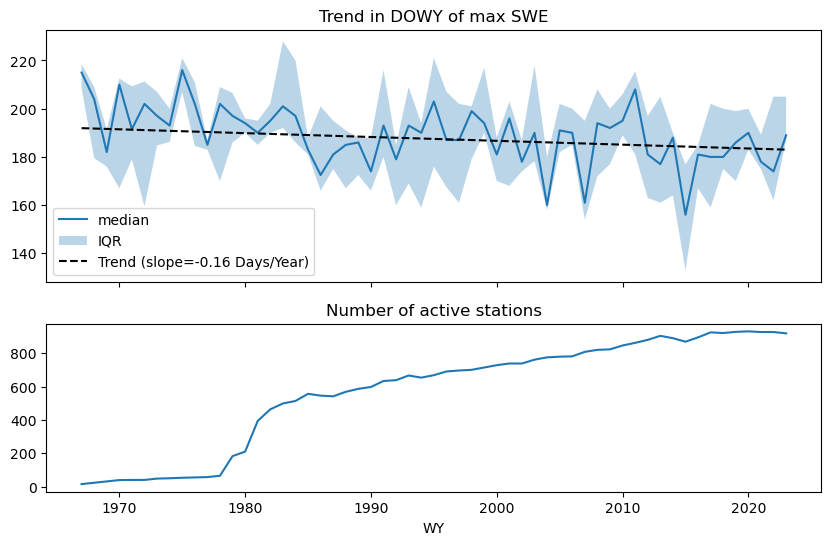
Calculate and plot trend in DOWY of max SWE for all data

• use DataFrame.groupby() to find the date of max SWE per year and convert to a DOWY value, store in all_stations_dowy_max_swe_df

• calculate slope and intercept of linear regression using np.polyfit() on a melted version of

• obtain statistics for each year using DataFrame.describe()

all_stations_dowy_max_swe_df = (
    all_stations_swe_df.groupby("WY").idxmax().map(easysnowdata.utils.datetime_to_DOWY)
)

stations_before_WY1982 = WesternUS.all_stations[WesternUS.all_stations.beginDate < "1981-10-01"]
dowy_max_swe_melted = pd.melt(
    all_stations_dowy_max_swe_df.reset_index(), id_vars="WY"
).dropna()
dowy_max_swe_melted_before_WY1982 = dowy_max_swe_melted[
    dowy_max_swe_melted["variable"].isin(stations_before_WY1982.index)
]
slope, intercept = np.polyfit(
    dowy_max_swe_melted_before_WY1982.WY, dowy_max_swe_melted_before_WY1982.value, 1
)
lr_years = np.unique(dowy_max_swe_melted.WY)

describe = all_stations_dowy_max_swe_df.T.describe()
describe

WY	1967.0	1968.0	1969.0	1970.0	1971.0	1972.0	1973.0	1974.0	1975.0	1976.0	...	2014.0	2015.0	2016.0	2017.0	2018.0	2019.0	2020.0	2021.0	2022.0	2023.0
count	15.000000	23.00000	31.000000	39.000000	40.000000	40.000000	48.000000	50.000000	53.000000	55.000000	...	891.000000	870.000000	896.000000	926.000000	922.000000	929.000000	932.000000	928.000000	928.000000	920.000000
mean	211.600000	196.73913	185.741935	197.641026	188.050000	186.375000	195.729167	195.720000	213.000000	194.800000	...	179.783389	156.452874	175.334821	179.018359	183.367679	185.812702	182.918455	180.346983	176.734914	192.546739
std	13.113788	19.17199	14.906302	25.243537	29.203047	33.502918	18.525129	17.996644	11.560876	18.673015	...	28.288029	36.552523	27.632212	25.712310	18.666580	19.338004	26.485426	18.764201	36.686443	13.905714
min	188.000000	170.00000	158.000000	148.000000	106.000000	94.000000	134.000000	161.000000	187.000000	154.000000	...	55.000000	33.000000	88.000000	104.000000	84.000000	95.000000	60.000000	119.000000	89.000000	86.000000
25%	208.500000	179.50000	176.000000	167.000000	179.000000	159.500000	184.750000	186.250000	207.000000	184.500000	...	164.000000	133.000000	167.000000	159.000000	175.000000	170.000000	183.000000	175.000000	162.000000	187.000000
50%	215.000000	204.00000	182.000000	210.000000	191.500000	202.000000	197.000000	193.000000	216.000000	202.000000	...	188.000000	156.000000	181.000000	180.000000	180.000000	186.000000	190.000000	178.000000	174.000000	189.000000
75%	218.500000	209.00000	191.500000	212.500000	209.250000	211.250000	207.000000	200.000000	221.000000	211.000000	...	190.000000	177.000000	185.000000	202.000000	200.000000	199.000000	200.000000	189.250000	205.000000	205.000000
max	228.000000	238.00000	219.000000	227.000000	235.000000	226.000000	225.000000	238.000000	240.000000	218.000000	...	238.000000	239.000000	232.000000	235.000000	224.000000	247.000000	229.000000	228.000000	250.000000	234.000000

8 rows × 57 columns

f, ax = plt.subplots(
    2, 1, figsize=(10, 6), sharex=True, gridspec_kw={"height_ratios": [3, 2]}
)

describe.loc["50%"].plot(ax=ax[0], label="median")

ax[0].fill_between(
    describe.columns, describe.loc["25%"], describe.loc["75%"], alpha=0.3, label="IQR"
)
ax[0].plot(
    lr_years,
    np.array(lr_years) * slope + intercept,
    "k--",
    label=f"Trend (slope={slope:.2f} Days/Year)",
)
# ax[0].set_xlim([1967,2023])

ax[0].legend()

describe.loc["count"].plot(ax=ax[1])


ax[0].set_title("Trend in DOWY of max SWE")
ax[1].set_title("Number of active stations")

Text(0.5, 1.0, 'Number of active stations')

Check out trend at each station seperately

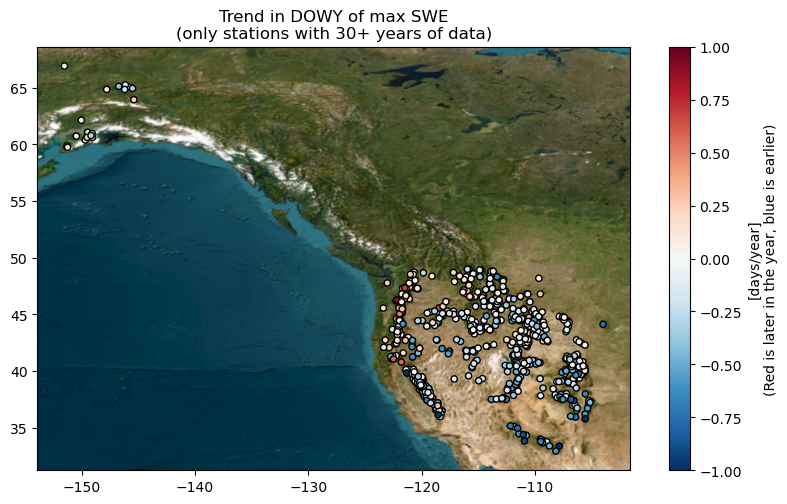
• calculate the linear trend in DOWY of max SWE only for stations with over 30 years of data, store in our original all_stations_gdf

  • out of 971 stations with SWE data, 645 meet this criteria

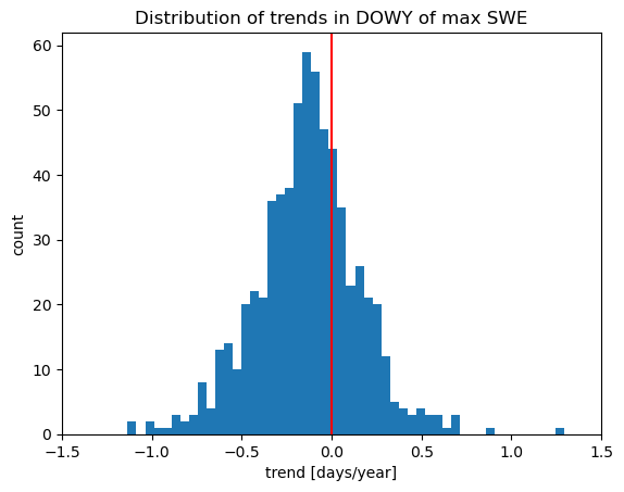
• plot the trend for each station and plot the trends on a histogram

WesternUS.all_stations.loc[:, "dowy_max_swe_trend"] = all_stations_dowy_max_swe_df.apply(
    lambda y: (
        np.polyfit(y.dropna().index.values, y.dropna(), 1)[0]
        if len(y.dropna()) >= 30
        else np.nan
    )
)

f, ax = plt.subplots(figsize=(10, 5.5))

WesternUS.all_stations.plot(
    column="dowy_max_swe_trend",
    ax=ax,
    legend=True,
    cmap="RdBu_r",
    edgecolor="k",
    markersize=20,
    vmin=-1,
    vmax=1,
    legend_kwds={"label": "[days/year]\n(Red is later in the year, blue is earlier)"},
)

ctx.add_basemap(
    ax, crs="EPSG:4326", source=ctx.providers.Esri.WorldImagery, attribution=""
)

ax.set_title("Trend in DOWY of max SWE\n(only stations with 30+ years of data)")

Text(0.5, 1.0, 'Trend in DOWY of max SWE\n(only stations with 30+ years of data)')

f, ax = plt.subplots()

ax.hist(WesternUS.all_stations["dowy_max_swe_trend"], bins=50)

ax.axvline(x=0, color="red")

ax.set_xlim([-1.5, 1.5])

ax.set_xlabel("trend [days/year]")
ax.set_ylabel("count")
ax.set_title("Distribution of trends in DOWY of max SWE")

Text(0.5, 1.0, 'Distribution of trends in DOWY of max SWE')

Let’s analyze these trends by mountain range

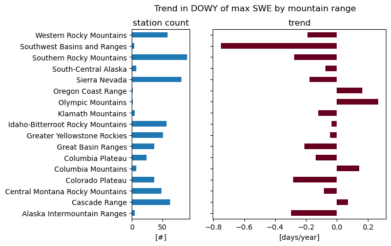
• we can DataFrame.groupby() our geodataframe by mountain range to calculate mountain range specific stats, store in mountain_range_trend_df

• mountain ranges with more stations (and more spatial coverage) are probably more trustworthy

mountain_range_count = (
    WesternUS.all_stations.dropna().groupby("mountainRange")["dowy_max_swe_trend"].count()
)
mountain_range_median = (
    WesternUS.all_stations.dropna().groupby("mountainRange")["dowy_max_swe_trend"].median()
)
mountain_range_mean = (
    WesternUS.all_stations.dropna().groupby("mountainRange")["dowy_max_swe_trend"].mean()
)
mountain_range_std = (
    WesternUS.all_stations.dropna().groupby("mountainRange")["dowy_max_swe_trend"].std()
)

mountain_range_trend_df = pd.concat(
    [
        mountain_range_count,
        mountain_range_median,
        mountain_range_mean,
        mountain_range_std,
    ],
    axis=1,
)
mountain_range_trend_df.columns = ["station_count", "median", "mean", "std"]

mountain_range_trend_df

	station_count	median	mean	std
mountainRange
Alaska Intermountain Ranges	5	-0.298031	-0.266592	0.112821
Cascade Range	63	0.072125	0.138312	0.346018
Central Montana Rocky Mountains	48	-0.083318	-0.100606	0.193399
Colorado Plateau	37	-0.282213	-0.348372	0.205635
Columbia Mountains	7	0.143695	0.082937	0.164431
Columbia Plateau	24	-0.138161	-0.029927	0.309255
Great Basin Ranges	37	-0.209381	-0.238700	0.206061
Greater Yellowstone Rockies	51	-0.044327	-0.064588	0.175889
Idaho-Bitterroot Rocky Mountains	57	-0.036092	-0.021299	0.242944
Klamath Mountains	5	-0.122516	0.019894	0.407079
Olympic Mountains	1	0.267235	0.267235	NaN
Oregon Coast Range	1	0.163264	0.163264	NaN
Sierra Nevada	81	-0.177622	-0.176293	0.283223
South-Central Alaska	7	-0.073497	-0.029532	0.230334
Southern Rocky Mountains	90	-0.275773	-0.277181	0.258862
Southwest Basins and Ranges	4	-0.752793	-0.740468	0.252450
Western Rocky Mountains	58	-0.191897	-0.171475	0.199642

f, ax = plt.subplots(1, 2, sharey=True, gridspec_kw={"width_ratios": [1, 3]})

mountain_range_trend_df["station_count"].plot.barh(ax=ax[0])
mountain_range_trend_df["median"].plot.barh(ax=ax[1], cmap="RdBu")


ax[0].set_xlabel("[#]")
ax[1].set_xlabel("[days/year]")
ax[0].set_ylabel("")
ax[0].set_title("station count")
ax[1].set_title("trend")

f.suptitle("Trend in DOWY of max SWE by mountain range")

Text(0.5, 0.98, 'Trend in DOWY of max SWE by mountain range')

Let’s visualize this on a map

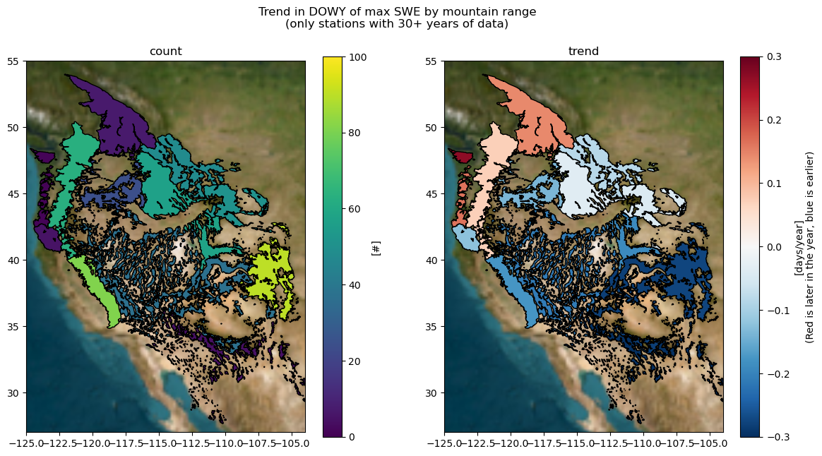
• add spatial information to mountain_range_trend_df using DataFrame.join() with mountain range geometries from GMBA Mountain Inventory v2

• ceate both a static plot with counts and medians and create an interactive plot so we can explore the trends across mountain ranges and stations

url = (
    f"https://data.earthenv.org/mountains/standard/GMBA_Inventory_v2.0_standard_300.zip"
)
gmba_gdf = gpd.read_file("zip+" + url)

mountain_range_trend_gdf = gpd.GeoDataFrame(
    mountain_range_trend_df.join(gmba_gdf[["MapName", "geometry"]].set_index("MapName"))
)

f, ax = plt.subplots(1, 2, figsize=(14, 7))

mountain_range_trend_gdf.plot(
    ax=ax[0],
    column="station_count",
    vmin=0,
    vmax=100,
    cmap="viridis",
    legend=True,
    edgecolor="k",
    legend_kwds={"label": "[#]"},
)
mountain_range_trend_gdf.plot(
    ax=ax[1],
    column="median",
    vmin=-0.3,
    vmax=0.3,
    cmap="RdBu_r",
    legend=True,
    edgecolor="k",
    legend_kwds={"label": "[days/year]\n(Red is later in the year, blue is earlier)"},
)

for axs in ax:
    ctx.add_basemap(
        ax=axs,
        crs=mountain_range_trend_gdf.crs,
        source=ctx.providers.Esri.WorldImagery,
        attribution=False,
    )
    ctx.add_basemap(
        ax=axs,
        crs=mountain_range_trend_gdf.crs,
        source=ctx.providers.Esri.WorldImagery,
        attribution=False,
    )
    axs.set_xlim([-125, -104])
    axs.set_ylim([27, 55])

ax[0].set_title("count")
ax[1].set_title("trend")

f.suptitle(
    "Trend in DOWY of max SWE by mountain range\n(only stations with 30+ years of data)"
)

Text(0.5, 0.98, 'Trend in DOWY of max SWE by mountain range\n(only stations with 30+ years of data)')

m = mountain_range_trend_gdf.explore(
    column="median", cmap="RdBu_r", vmin=-0.5, vmax=0.5
)
WesternUS.all_stations.astype(dict(beginDate=str, endDate=str)).explore(
    m=m, column="dowy_max_swe_trend", cmap="RdBu_r", vmin=-0.3, vmax=0.3
)

Make this Notebook Trusted to load map: File -> Trust Notebook

Looks like these trends are different by region, but relatively consistent within region. The majority of regions show the timing of maximum SWE happening earlier in the year, with notable exceptions being mountain ranges in the Pacific Northwest which show a reverse trend with smaller magnitude. Also of importance is the number of stations and their spatial dsitribution in each region, as 2 of the 4 regions (Olympic Mountains and Oregon Coast Range) showing the timing of maximum SWE happening later in the year only have one station each with a 30+ year record.

What if we want to check out all available daily variables at all SNOTEL and CCSS stations for all time?

• Let’s check the data out as an xarray object!

AllStations = easysnowdata.automatic_weather_stations.StationCollection()

Geodataframe with all stations has been added to the Station object. Please use the .all_stations attribute to access.
Use the .get_data(stations=geodataframe/string/list,variables=string/list,start_date=str,end_date=str) method to fetch data for specific stations and variables.

AllStations.get_entire_data_archive()

Downloading compressed data to a temporary directory (/tmp/all_station_data.tar.lzma)...
Decompressing data...
Creating xarray.Dataset from the uncompressed data...
Done! Entire archive dataset has been added to the station object. Please use the .entire_data_archive attribute to access.

AllStations.entire_data_archive

<xarray.Dataset> Size: 1GB
Dimensions:        (time: 23826, station: 969)
Coordinates: (12/16)
  * time           (time) datetime64[ns] 191kB 1909-04-13 ... 2024-03-17
    name           (station) <U24 93kB 'New Crescent Lake' ... 'Paradise Meadow'
    network        (station) <U6 23kB 'SNOTEL' 'SNOTEL' ... 'CCSS' 'CCSS'
    elevation_m    (station) float64 8kB 1.497e+03 2.621e+03 ... 2.332e+03
    latitude       (station) float64 8kB 43.51 40.21 37.65 ... 38.48 39.62 38.05
    longitude      (station) float64 8kB -122.0 -105.6 -107.8 ... -120.7 -119.7
    ...             ...
    beginDate      (station) datetime64[ns] 8kB 1979-10-01 ... 2005-10-01
    endDate        (station) datetime64[ns] 8kB 2024-04-03 ... 2024-04-03
    csvData        (station) bool 969B True True True True ... True True True
    geometry       (station) object 8kB POINT (-121.97982025146484 43.5118484...
    WY             (time) int64 191kB 1909 1955 1955 1955 ... 2024 2024 2024
    DOWY           (time) int64 191kB 195 62 63 64 65 66 ... 165 166 167 168 169
Dimensions without coordinates: station
Data variables:
    TAVG           (station, time) float64 185MB nan nan nan ... -1.1 0.0 nan
    TMIN           (station, time) float64 185MB nan nan nan ... -3.9 -5.0 nan
    TMAX           (station, time) float64 185MB nan nan nan nan ... 3.3 7.2 nan
    SNWD           (station, time) float64 185MB nan nan nan ... 2.286 2.235
    WTEQ           (station, time) float64 185MB nan nan nan ... 0.8352 0.8354
    PRCPSA         (station, time) float64 185MB nan nan nan nan ... nan nan nan

xarray.Dataset

• Dimensions:
  • time: 23826
  • station: 969
• Coordinates: (16)
  • time
    (time)
    datetime64[ns]
    1909-04-13 ... 2024-03-17

    array(['1909-04-13T00:00:00.000000000', '1954-12-01T00:00:00.000000000',
           '1954-12-02T00:00:00.000000000', ..., '2024-03-15T00:00:00.000000000',
           '2024-03-16T00:00:00.000000000', '2024-03-17T00:00:00.000000000'],
          dtype='datetime64[ns]')

  • name
    (station)
    <U24
    'New Crescent Lake' ... 'Paradis...

    array(['New Crescent Lake', 'Copeland Lake', 'Cascade', 'Mount Gardner',
           'Tamarack Summit', 'Fairbanks F.O.', 'Saddle Mountain',
           'Lake Lois', 'Calvert Creek', 'Timber Creek', 'Trial Lake',
           'ONeil Creek', 'Bloody Dick', 'Ivanhoe', 'Ebbetts Pass',
           'Redden Mine Lwr', 'East Rim Divide', 'Upper Burnt Corral',
           'Santiam Jct.', 'Cloud Peak Reservoir', 'Ward Mountain',
           'Lower Kibbie Ridge', 'Burts Miller Ranch', 'Cold Springs',
           'Beaver Head', 'Timberline', 'Windy Peak', 'Frohner Meadow',
           'Virginia Lakes Ridge', 'Calamity', 'Garver Creek',
           'Mt Rose Ski Area', 'Trinchera', 'Mores Creek Summit', 'Golconda',
           'Thaynes Canyon', 'Buffalo Park', 'Red Rock Mountain', 'Dry Lake',
           'Cayuse Pass', 'Clayton Springs', 'Casa Vieja Meadows',
           'Cole Canyon', 'Heber', 'Trinity', 'Gooseberry RS', 'Vacas Locas',
           'Lost-Wood Divide', 'Rabbit Ears', 'Takka Wiiya', 'Blacktail Mtn',
           'Buckboard Flat', 'Schofield Pass', 'Slagamelt Lakes',
           'Gianelli Meadow', 'Parrish Creek', 'Big Goose', 'Blazed Alder',
           'Fry', 'Dana Meadows', 'Upper Nome Creek', 'Meadow Lake',
           'Smiley Mountain', 'Beach Meadows', 'Clackamas Lake', 'Marquette',
           'Sheep Mtn.', 'George Creek', 'Little Meadows',
           'Red River Pass #2', 'Silver Creek Divide', 'Bear Creek',
    ...
           'Emigrant Summit', 'Lone Mountain', 'Beaver Creek', 'Indian Pass',
           'Dupuyer Creek', 'Spratt Creek', 'Beaver Divide', 'Barker Lakes',
           'Red Mountain Pass', 'Paradise', 'Soldier Park', 'Tower',
           'Lewis Lake Divide', 'Currant Creek', 'Forestdale Creek',
           'Panguitch Lake RS', 'Snow Mountain', 'Smith  Morehouse',
           'Molas Lake', 'Marlette Lake', 'Copper Camp', 'Carrot Basin',
           'Whiskey Park', 'Daniels-Strawberry', 'Fisher Creek',
           'Bear Canyon', 'Mill Creek Summit', 'Columbine Pass',
           'Loomis Park', 'Taos Powderhorn', 'Heen Latinee', 'MF Nooksack',
           'Spruce Springs', 'Cent Sierra Snow Lab',
           'Tioga Pass Entry Station', 'Cascade Mountain', 'Galena Summit',
           'Bostetter R.S.', 'Red Hill', 'Frisco Divide', 'Diamond Peak',
           'Box Canyon', 'Seine Creek', 'Quartz Peak', 'Galena', 'Muckamuck',
           'Mcknight Cabin', 'Hayden Pass', 'Trapper Lake', 'Parker Peak',
           'Lone Cone', 'Deadman Creek', 'Heavenly Valley', 'Bison Lake',
           'Rock Creek', 'Thumb Divide', 'Four Trees', 'Indian Canyon',
           'Baker Butte', 'Morgan Creek', 'Caples Lake', 'Kimberly Mine',
           'Touchet', 'Kalamazoo', 'Upper San Juan', 'Mc Clure Pass',
           'Lasal Mountain', 'Robinson Cow Camp', 'Paradise Meadow'],
          dtype='<U24')

  • network
    (station)
    <U6
    'SNOTEL' 'SNOTEL' ... 'CCSS' 'CCSS'

    array(['SNOTEL', 'SNOTEL', 'SNOTEL', 'SNOTEL', 'CCSS', 'SNOTEL', 'SNOTEL',
           'CCSS', 'SNOTEL', 'SNOTEL', 'SNOTEL', 'SNOTEL', 'SNOTEL', 'SNOTEL',
           'CCSS', 'SNOTEL', 'SNOTEL', 'CCSS', 'SNOTEL', 'SNOTEL', 'SNOTEL',
           'CCSS', 'SNOTEL', 'SNOTEL', 'SNOTEL', 'SNOTEL', 'SNOTEL', 'SNOTEL',
           'CCSS', 'SNOTEL', 'SNOTEL', 'SNOTEL', 'SNOTEL', 'SNOTEL', 'SNOTEL',
           'SNOTEL', 'SNOTEL', 'CCSS', 'SNOTEL', 'SNOTEL', 'SNOTEL', 'CCSS',
           'SNOTEL', 'SNOTEL', 'SNOTEL', 'SNOTEL', 'SNOTEL', 'SNOTEL',
           'SNOTEL', 'SNOTEL', 'SNOTEL', 'SNOTEL', 'SNOTEL', 'SNOTEL', 'CCSS',
           'SNOTEL', 'SNOTEL', 'SNOTEL', 'SNOTEL', 'CCSS', 'SNOTEL', 'SNOTEL',
           'SNOTEL', 'CCSS', 'SNOTEL', 'SNOTEL', 'SNOTEL', 'SNOTEL', 'SNOTEL',
           'SNOTEL', 'SNOTEL', 'SNOTEL', 'CCSS', 'SNOTEL', 'SNOTEL', 'SNOTEL',
           'SNOTEL', 'SNOTEL', 'SNOTEL', 'SNOTEL', 'SNOTEL', 'SNOTEL',
           'SNOTEL', 'SNOTEL', 'SNOTEL', 'SNOTEL', 'SNOTEL', 'SNOTEL',
           'SNOTEL', 'SNOTEL', 'SNOTEL', 'SNOTEL', 'CCSS', 'CCSS', 'CCSS',
           'SNOTEL', 'SNOTEL', 'SNOTEL', 'SNOTEL', 'CCSS', 'SNOTEL', 'SNOTEL',
           'SNOTEL', 'SNOTEL', 'SNOTEL', 'SNOTEL', 'SNOTEL', 'CCSS', 'SNOTEL',
           'SNOTEL', 'SNOTEL', 'SNOTEL', 'SNOTEL', 'SNOTEL', 'SNOTEL',
           'SNOTEL', 'SNOTEL', 'SNOTEL', 'SNOTEL', 'SNOTEL', 'SNOTEL',
           'SNOTEL', 'SNOTEL', 'SNOTEL', 'SNOTEL', 'SNOTEL', 'SNOTEL', 'CCSS',
           'SNOTEL', 'CCSS', 'SNOTEL', 'SNOTEL', 'SNOTEL', 'SNOTEL', 'SNOTEL',
    ...
           'SNOTEL', 'SNOTEL', 'SNOTEL', 'SNOTEL', 'SNOTEL', 'SNOTEL',
           'SNOTEL', 'SNOTEL', 'SNOTEL', 'SNOTEL', 'CCSS', 'SNOTEL', 'SNOTEL',
           'SNOTEL', 'SNOTEL', 'SNOTEL', 'SNOTEL', 'SNOTEL', 'SNOTEL',
           'SNOTEL', 'CCSS', 'SNOTEL', 'SNOTEL', 'SNOTEL', 'SNOTEL', 'SNOTEL',
           'CCSS', 'CCSS', 'SNOTEL', 'CCSS', 'CCSS', 'SNOTEL', 'SNOTEL',
           'SNOTEL', 'SNOTEL', 'CCSS', 'SNOTEL', 'SNOTEL', 'SNOTEL', 'SNOTEL',
           'SNOTEL', 'CCSS', 'SNOTEL', 'SNOTEL', 'SNOTEL', 'SNOTEL', 'SNOTEL',
           'CCSS', 'CCSS', 'SNOTEL', 'SNOTEL', 'SNOTEL', 'SNOTEL', 'SNOTEL',
           'SNOTEL', 'SNOTEL', 'SNOTEL', 'SNOTEL', 'SNOTEL', 'SNOTEL',
           'SNOTEL', 'SNOTEL', 'SNOTEL', 'SNOTEL', 'SNOTEL', 'CCSS', 'SNOTEL',
           'SNOTEL', 'SNOTEL', 'SNOTEL', 'SNOTEL', 'SNOTEL', 'SNOTEL',
           'SNOTEL', 'SNOTEL', 'SNOTEL', 'CCSS', 'SNOTEL', 'SNOTEL', 'SNOTEL',
           'SNOTEL', 'SNOTEL', 'SNOTEL', 'SNOTEL', 'SNOTEL', 'SNOTEL',
           'SNOTEL', 'SNOTEL', 'SNOTEL', 'SNOTEL', 'SNOTEL', 'SNOTEL',
           'SNOTEL', 'CCSS', 'CCSS', 'SNOTEL', 'SNOTEL', 'SNOTEL', 'SNOTEL',
           'SNOTEL', 'SNOTEL', 'SNOTEL', 'SNOTEL', 'SNOTEL', 'SNOTEL',
           'SNOTEL', 'SNOTEL', 'SNOTEL', 'SNOTEL', 'SNOTEL', 'SNOTEL', 'CCSS',
           'SNOTEL', 'SNOTEL', 'SNOTEL', 'SNOTEL', 'CCSS', 'SNOTEL', 'SNOTEL',
           'SNOTEL', 'CCSS', 'SNOTEL', 'SNOTEL', 'SNOTEL', 'SNOTEL', 'SNOTEL',
           'SNOTEL', 'CCSS', 'CCSS'], dtype='<U6')

  • elevation_m
    (station)
    float64
    1.497e+03 2.621e+03 ... 2.332e+03

    array([1496.56799316, 2621.2800293 , 2706.62402344,  890.01599121,
           2301.24      ,  137.16000366,  947.92797852, 2621.28      ,
           1959.86401367, 2423.15991211, 3045.56152344, 1987.29602051,
           2316.47998047, 3169.91992188, 2651.76      , 2600.55371094,
           2417.06396484, 2956.56      , 1139.95202637, 3005.32788086,
           2804.15991211, 2042.16      , 2438.39990234, 2935.22412109,
           2435.35205078, 2662.73291016, 2407.91992188, 1975.10400391,
           2834.64      ,  762.        , 1295.40002441, 2682.54492188,
           3310.12792969, 1859.2800293 , 2016.5567627 , 2813.30395508,
           2816.35205078, 2042.16      , 2560.32006836, 1597.15197754,
           3062.93530273, 2529.84      , 1801.36804199, 2328.67211914,
            893.06402588, 2421.33129883, 2836.46875   , 2407.91992188,
           2865.12011719, 2780.38549805, 1722.11999512, 2720.03515625,
           3261.36010742, 2627.37597656, 2560.32      , 2359.15209961,
           2435.35205078, 1112.52001953, 2194.56005859, 2987.04      ,
            768.0960083 , 2788.91992188, 2901.69604492, 2331.72      ,
           1036.31994629, 2670.0480957 , 2026.92004395, 2732.22729492,
           1225.29602051, 3002.2800293 , 2743.19995117, 2450.59204102,
           1645.92      , 3048.        , 2651.76000977, 1271.01599121,
           2248.50952148, 2112.26391602,  868.67999268,  426.72000122,
    ...
           2901.08642578, 2451.8112793 ,  213.36000061, 2662.12329102,
           2621.2800293 , 2578.60791016, 2334.76806641, 3020.56811523,
           2252.47192383, 2706.62402344, 2392.67993164,  716.2800293 ,
           1752.59997559, 1874.52      , 2523.74389648, 2514.60009766,
           3413.76000977, 1563.62402344, 2657.85595703, 3200.39990234,
           2392.67993164, 2412.49194336, 2443.58154297, 2545.08007812,
           1813.56      , 2325.92871094, 3200.39990234, 2403.04321289,
           2118.36010742, 2743.19995117, 2727.95996094, 2440.83837891,
           2773.67993164, 2407.91992188, 2682.23999023, 2865.12011719,
           2511.55200195, 3370.17358398,  629.4119873 , 1514.85595703,
           1737.35998535, 2103.12      , 3031.236     , 2369.51513672,
           2676.14404297, 2286.        , 1344.16796875, 2438.39990234,
           2443.58154297, 2033.01599121,  627.88800049, 1432.56005859,
           2276.85595703, 1362.45605469, 2816.35205078, 3267.45605469,
           2956.56005859, 2865.12011719, 2926.08007812, 2819.4       ,
           2601.16308594, 3316.22412109, 2403.65283203, 2432.30395508,
           1585.5696    , 2795.32080078, 2225.04003906, 2316.47998047,
           2438.4       , 2773.98486328, 1685.54394531, 2369.82006836,
           3108.95996094, 2895.60009766, 2919.37451172, 1975.104     ,
           2331.72      ])

  • latitude
    (station)
    float64
    43.51 40.21 37.65 ... 39.62 38.05

    array([43.51184845, 40.20777893, 37.65082932, 47.35768127, 37.16375   ,
           64.84999847, 45.54476929, 38.921036  , 45.88380051, 44.02740097,
           40.6780014 , 41.86420059, 45.16506958, 39.29201889, 38.561     ,
           40.67504883, 43.13097   , 37.183296  , 44.43503189, 44.40343094,
           39.13241959, 38.033024  , 40.9849205 , 43.2767601 , 33.69144058,
           39.67712021, 42.28020096, 46.43545151, 38.077     , 45.90362167,
           48.97523117, 39.31573105, 37.35327911, 43.93199921, 40.88357925,
           40.62350082, 40.22861099, 41.023621  , 40.53396988, 46.86954117,
           37.97249985, 36.198097  , 44.4863205 , 34.31201935, 48.0746994 ,
           38.80033875, 36.02634811, 43.82432175, 40.36782837, 39.74103928,
           47.98287964, 37.86943054, 39.01522064, 45.36526108, 38.204308  ,
           40.93416977, 44.57923889, 45.42869949, 35.07297134, 37.896162  ,
           65.36710358, 44.43655014, 43.72718048, 36.126095  , 45.09658051,
           44.30160141, 43.21030045, 41.9156189 , 44.61296844, 36.69924927,
           33.37105942, 41.83383942, 41.16914   , 36.71630859, 39.29721832,
           47.04439926, 40.18537903, 41.75067139, 65.09999847, 60.61713028,
           46.92832947, 44.14424896, 44.57461929, 40.53215027, 42.86983871,
           45.17367172, 48.1747818 , 45.98210144, 42.43582916, 39.25259018,
           46.54740906, 45.18832016, 41.237     , 39.001     , 38.932     ,
           44.12612152, 38.85189819, 60.39027023, 42.76477814, 38.943947  ,
    ...
           38.8365    , 39.23802948, 44.71960831, 48.15678024, 48.19797897,
           37.457275  , 41.22869873, 61.11483002, 45.24010086, 38.99076843,
           48.12672043, 38.7194    , 35.70429993, 48.95159912, 46.84233856,
           45.50381088, 43.11265182, 41.591389  , 38.318     , 39.30229187,
           48.69092178, 38.50809097, 40.73899841, 39.92975998, 60.25965118,
           38.8818512 , 45.01787949, 35.23332977, 42.70991898, 40.03522873,
           42.36054993, 45.27412033, 44.94966125, 61.06766891, 48.06341171,
           38.66627   , 40.61233139, 46.09712982, 37.89179993, 46.78264999,
           44.34846878, 40.53742981, 44.20861816, 40.35747147, 38.68244934,
           37.70463181, 40.778809  , 40.78931046, 37.74932098, 39.16395187,
           47.08158112, 44.96192169, 41.00289154, 40.29529953, 45.06235123,
           43.74367142, 44.47211838, 38.41794968, 43.17387009, 36.58203125,
           58.69652176, 48.82453156, 46.18286896, 39.325     , 37.91087   ,
           40.28300095, 43.87496948, 42.16442108, 45.46429825, 33.73646164,
           39.56361008, 45.27190018, 45.52687836, 47.87926865, 43.87722015,
           48.58525848, 33.00812149, 38.29325867, 39.99884033, 44.7339592 ,
           37.89183044, 38.331596  , 38.92430878, 39.76486969, 40.54875183,
           44.36917114, 39.81278   , 39.89165878, 34.45660019, 44.84236908,
           38.710793  , 38.4838295 , 46.11867905, 39.55789948, 37.48575974,
           39.1289711 , 38.48226166, 39.621864  , 38.046117  ])

  • longitude
    (station)
    float64
    -122.0 -105.6 ... -120.7 -119.7

    array([-121.97982025, -105.56861115, -107.80602264, -121.56812286,
           -119.200531  , -147.80000305, -123.37315369, -120.204445  ,
           -113.32553101, -109.17878723, -110.94873047, -115.0831604 ,
           -113.50099182, -106.54923248, -119.808     , -111.21765137,
           -110.20230103, -118.938293  , -121.94502258, -107.06056976,
           -114.95574951, -119.879245  , -110.85075378, -109.44584656,
           -109.21656799, -110.43395233, -105.57816315, -112.19277191,
           -119.234     , -122.21633148, -115.81915283, -119.89472961,
           -105.23233032, -115.6658783 , -117.58811951, -111.53321838,
           -106.59528351, -122.886627  , -106.78130341, -121.53430176,
           -111.8335495 , -118.267685  , -104.41056824, -110.75431061,
           -120.84929657, -111.68332672, -106.81362152, -114.26402283,
           -106.74037933, -113.98262024, -114.35430145, -109.44716644,
           -107.04876709, -113.71833801, -119.893188  , -111.8137207 ,
           -107.20068359, -121.85604858, -111.84374237, -119.25726   ,
           -146.59199524, -113.31815338, -113.83402252, -118.293457  ,
           -121.75443268, -109.2401886 , -111.68791962, -113.41153717,
           -122.22564697, -105.34124756, -108.70617676, -115.45278168,
           -121.939827  , -106.26348114, -106.60694122, -121.94032288,
           -111.35971069, -117.5318222 , -144.9331665 , -149.53128052,
    ...
           -109.67279816, -111.63108826, -149.34228516, -112.24915314,
           -111.84559631, -108.26667023, -118.63210297, -105.54425812,
           -111.56085205, -111.42691803, -111.35852051, -149.47950745,
           -112.75730133, -119.81742   , -111.09781647, -113.13037872,
           -107.71341705, -121.74765015, -107.01360321, -106.67680359,
           -110.66628265, -111.08992767, -119.95970154, -112.65036774,
           -121.782677  , -111.09191895, -107.68865967, -119.89672089,
           -112.72955322, -111.29402924, -106.90847778, -111.25676727,
           -109.94487762, -113.93797302, -114.48992157, -108.38249207,
           -110.14006805, -105.45610809, -134.86448669, -121.92951202,
           -117.54154968, -120.367     , -119.258507  , -111.60991669,
           -114.71363068, -114.19271851, -121.70427704, -108.94502258,
           -115.84420776, -110.24903107, -123.29856873, -117.08937836,
           -114.67250061, -119.86624146, -107.86975098, -105.85050201,
           -107.23619843, -109.9148407 , -108.1954422 , -119.654114  ,
           -119.91641235, -107.35681152, -110.69291687, -110.57717133,
           -121.32168   , -110.74604034, -111.40643311, -114.26870728,
           -120.04158   , -112.39273071, -117.85050201, -114.62761688,
           -106.83535004, -107.28806305, -109.27198029, -120.679871  ,
           -119.671748  ])

  • state
    (station)
    <U12
    'Oregon' ... 'California'

    array(['Oregon', 'Colorado', 'Colorado', 'Washington', 'California',
           'Alaska', 'Oregon', 'California', 'Montana', 'Wyoming', 'Utah',
           'Nevada', 'Montana', 'Colorado', 'California', 'Utah', 'Wyoming',
           'California', 'Oregon', 'Wyoming', 'Nevada', 'California', 'Utah',
           'Wyoming', 'Arizona', 'Utah', 'Wyoming', 'Montana', 'California',
           'Washington', 'Montana', 'Nevada', 'Colorado', 'Idaho', 'Nevada',
           'Utah', 'Colorado', 'California', 'Colorado', 'Washington', 'Utah',
           'California', 'Wyoming', 'Arizona', 'Washington', 'Utah',
           'New Mexico', 'Idaho', 'Colorado', 'Utah', 'Montana', 'Utah',
           'Colorado', 'Montana', 'California', 'Utah', 'Wyoming', 'Oregon',
           'Arizona', 'California', 'Alaska', 'Idaho', 'Idaho', 'California',
           'Oregon', 'Wyoming', 'Idaho', 'Utah', 'Oregon', 'New Mexico',
           'New Mexico', 'Nevada', 'California', 'New Mexico', 'Colorado',
           'Washington', 'Utah', 'Nevada', 'Alaska', 'Alaska', 'Washington',
           'Oregon', 'Wyoming', 'Colorado', 'Wyoming', 'Montana', 'Montana',
           'Oregon', 'Wyoming', 'Nevada', 'Washington', 'Oregon',
           'California', 'California', 'California', 'Wyoming', 'California',
           'Alaska', 'Idaho', 'California', 'Oregon', 'Utah', 'Montana',
           'Idaho', 'Oregon', 'Oregon', 'Montana', 'California', 'Washington',
           'Montana', 'Utah', 'Oregon', 'Wyoming', 'Alaska', 'Utah',
    ...
           'California', 'Utah', 'Montana', 'Utah', 'Idaho', 'New Mexico',
           'California', 'California', 'Idaho', 'California', 'California',
           'Utah', 'Wyoming', 'Montana', 'Washington', 'California', 'Nevada',
           'Alaska', 'Montana', 'Colorado', 'Montana', 'California',
           'New Mexico', 'Washington', 'Montana', 'Montana', 'Wyoming',
           'California', 'California', 'Utah', 'Washington', 'Utah', 'Utah',
           'Utah', 'Alaska', 'Utah', 'Montana', 'New Mexico', 'Oregon',
           'Colorado', 'Idaho', 'Montana', 'Montana', 'Alaska', 'Montana',
           'California', 'Utah', 'Montana', 'Colorado', 'Washington',
           'Wyoming', 'Colorado', 'Wyoming', 'Utah', 'California', 'Utah',
           'California', 'Utah', 'Colorado', 'Nevada', 'Montana', 'Montana',
           'Wyoming', 'Utah', 'Montana', 'Idaho', 'Idaho', 'Colorado',
           'Wyoming', 'New Mexico', 'Alaska', 'Washington', 'Washington',
           'California', 'California', 'Utah', 'Idaho', 'Idaho', 'Oregon',
           'New Mexico', 'Nevada', 'Montana', 'Oregon', 'Washington', 'Idaho',
           'Washington', 'New Mexico', 'Colorado', 'Colorado', 'Wyoming',
           'Colorado', 'California', 'California', 'Colorado', 'Utah',
           'Wyoming', 'California', 'Utah', 'Arizona', 'Idaho', 'California',
           'Utah', 'Washington', 'Nevada', 'Colorado', 'Colorado', 'Utah',
           'California', 'California'], dtype='<U12')

  • HUC
    (station)
    <U12
    '170703020205' ... '180400090503'

    array(['170703020205', '101900050202', '140801040201', '171100120103',
           '180400060903', '190803060907', '170900100201', '180201280201',
           '100200040801', '100800090210', '160202030102', '170402130106',
           '100200011002', '140100040501', '160502010104', '160201010103',
           '170401030203', '180300100603', '170900040201', '100902060301',
           '150100110105', '180400090303', '160101010105', '100800010702',
           '150601010107', '140600070903', '101800080802', '100301011305',
           '160503010103', '170800020603', '170101030202', '160501020304',
           '130100020601', '170501110503', '160401080102', '160201020101',
           '140100010706', '180102110501', '140500010409', '171100140301',
           '160300020501', '180300010401', '101202030302', '150200100201',
           '170200110302', '160300030405', '130202020102', '170402190304',
           '140500010402', '160203060804', '170102080302', '140802030103',
           '140100040701', '100200040308', '180400100501', '160201020501',
           '100901010103', '170800010102', '150602020501', '180400090102',
           '190804020304', '170602040101', '170402180102', '180300010403',
           '170900110301', '100800130303', '170402050304', '170402100401',
           '170900060301', '130201010301', '150400040605', '170501020301',
           '180200040208', '130201021401', '140100040504', '171100140103',
           '160202020304', '160401090502', '190803060102', '190203020401',
    ...
           '140600100802', '160202020601', '190203020902', '160300051307',
           '100200070803', '130202070203', '171200030107', '101900050401',
           '160102020206', '100200080201', '100200070402', '190203020701',
           '100302010501', '160502010107', '160202030105', '170102010304',
           '140801040103', '171100150104', '100902060103', '140500010407',
           '170401010104', '140600040401', '160502010301', '160300010402',
           '180200031103', '160201010203', '140801040302', '160501010201',
           '170102030103', '100200080105', '140500030102', '140600040101',
           '100700060202', '170402180101', '170602010501', '140200050202',
           '140401010201', '130201010701', '190103010401', '171100040303',
           '170601030201', '180201250602', '180400090102', '160202030505',
           '170402190101', '170402120201', '170701050505', '150400040303',
           '160600051503', '100700020902', '170900100203', '170103080302',
           '170402190101', '170200062001', '130302020103', '130100030301',
           '140500050101', '100700010502', '140300030302', '180400100203',
           '160501010302', '140100011401', '140600030304', '100700010409',
           '180201210801', '140600040701', '150602030206', '170602030901',
           '180201290101', '160300030104', '170701020303', '160600080700',
           '140801010203', '140200040203', '140300050404', '180201250102',
           '180400090503'], dtype='<U12')

  • mgrs
    (station)
    <U5
    '10TEP' '13TDE' ... '10SFJ' '11SKC'

    array(['10TEP', '13TDE', '13SBB', '10TFT', '11SLB', '06WVS', '10TDR',
           '10SGJ', '12TUR', '12TXP', '12TWL', '11TPG', '12TUR', '13SCD',
           '11SKC', '12TVL', '12TWN', '11SLB', '10TEQ', '13TCK', '11SPD',
           '11SKC', '12TWL', '12TXN', '12SXC', '12SWJ', '13TDG', '12TVS',
           '11SLC', '10TER', '11UNQ', '11SKD', '13SDB', '11TPJ', '11TMF',
           '12TVK', '13TCE', '10TEL', '13TCE', '10TFS', '12SVH', '11SLA',
           '13TEK', '12SWC', '10UFU', '12SVH', '13SCV', '11TQJ', '13TCE',
           '12STK', '11TPP', '12SXG', '13SCD', '12TTR', '11SKC', '12TVL',
           '13TCK', '10TER', '12SVD', '11SLB', '06WWT', '12TUQ', '12TTP',
           '11SLV', '10TEQ', '12TXQ', '12TVN', '12TUM', '10TEQ', '13SDA',
           '12SYB', '11TPG', '10TEL', '13SCA', '13SCD', '10TET', '12TVK',
           '11TMG', '06WWT', '06VUN', '10TES', '10TFP', '13TCK', '13TDE',
           '12TXN', '12TTR', '12UXU', '11TML', '13TDG', '11SKD', '10TFS',
           '10TFR', '10TFL', '10SGJ', '10SGJ', '12TWP', '11SKD', '06VUM',
           '11TNH', '10SGJ', '10TEQ', '12STG', '12UUU', '11TNK', '11TLK',
           '11TKK', '12TVS', '11SKB', '11ULQ', '12TVR', '12SVJ', '11TMK',
           '13TCF', '05VMH', '12SVH', '13SCC', '12TVL', '10UFU', '10TFT',
           '12TTT', '10UEV', '10TFM', '11TPF', '13SDD', '13TCF', '11UNP',
           '12TWQ', '10SGH', '11TPG', '10SGJ', '13TCF', '12TVQ', '13TDF',
           '11TPE', '12SYG', '12SVJ', '12SUG', '10TFT', '11TNK', '12STG',
    ...
           '13SCD', '10UFU', '11SKD', '13SCC', '12TUS', '13TCK', '11TLL',
           '13TCK', '10TFS', '13SCC', '13SCB', '11SPA', '12TVM', '13TCK',
           '13TDE', '10TEN', '12SWC', '11SLB', '12SUG', '11TPG', '10UFU',
           '10TEQ', '10TFT', '10SGJ', '13SDV', '12SVD', '12TTT', '11SKC',
           '12TWL', '12TUQ', '12SUG', '11TPM', '13SDA', '10SGH', '11SKB',
           '11TNJ', '11SKB', '11SKD', '12SVJ', '12TWQ', '12UTU', '10UFU',
           '11SLB', '11TNF', '06VUN', '12TXR', '13SCD', '11UPP', '11SKC',
           '13SDV', '11ULQ', '12TUS', '12TWR', '12TWN', '10TFM', '11SKC',
           '12SVJ', '10UEU', '12SVH', '12TXL', '12SVK', '06VUM', '12SUJ',
           '12TVQ', '12SYE', '11TLH', '13TDE', '12TVM', '12TVR', '12TVQ',
           '06VUN', '12UUU', '11SKC', '12TVK', '12TUS', '13SBB', '10TES',
           '13TCK', '13TCE', '12TWP', '12TVK', '11SKC', '12SUG', '10TFL',
           '12TVL', '13SBB', '11SKD', '12TUT', '12TVQ', '13TCF', '12TVK',
           '12TWQ', '12TTP', '11TPK', '12SYH', '12TWN', '13SDA', '08VNL',
           '10UEV', '11TMM', '10SGJ', '11SLB', '12TVK', '11TPJ', '11TQG',
           '10TFR', '12SXC', '11SND', '12TWR', '10TDR', '11TMP', '11TPJ',
           '11UKP', '13SBS', '13SDC', '13SCE', '12TWQ', '12SYG', '11SKC',
           '11SKD', '13SBE', '12TWK', '12TWQ', '10SFK', '12SWK', '12SVD',
           '11TQK', '10SGH', '12SUH', '11TMM', '11SQD', '13SCB', '13SCD',
           '12SXH', '10SFJ', '11SKC'], dtype='<U5')

  • mountainRange
    (station)
    object
    'Cascade Range' ... 'Sierra Nevada'

    array(['Cascade Range', 'Southern Rocky Mountains',
           'Southern Rocky Mountains', 'Cascade Range', 'Sierra Nevada', None,
           'Oregon Coast Range', 'Sierra Nevada', None,
           'Greater Yellowstone Rockies', 'Western Rocky Mountains',
           'Great Basin Ranges', 'Idaho-Bitterroot Rocky Mountains',
           'Southern Rocky Mountains', 'Sierra Nevada',
           'Western Rocky Mountains', None, 'Sierra Nevada', 'Cascade Range',
           'Greater Yellowstone Rockies', 'Great Basin Ranges',
           'Sierra Nevada', None, 'Greater Yellowstone Rockies',
           'Colorado Plateau', 'Colorado Plateau', 'Southern Rocky Mountains',
           'Central Montana Rocky Mountains', 'Sierra Nevada',
           'Cascade Range', 'Columbia Mountains', 'Sierra Nevada',
           'Southern Rocky Mountains', 'Idaho-Bitterroot Rocky Mountains',
           'Great Basin Ranges', 'Western Rocky Mountains',
           'Southern Rocky Mountains', 'Klamath Mountains',
           'Southern Rocky Mountains', 'Cascade Range', None, 'Sierra Nevada',
           'Black Hills', None, 'Cascade Range', 'Colorado Plateau',
           'Colorado Plateau', 'Idaho-Bitterroot Rocky Mountains',
           'Southern Rocky Mountains', 'Great Basin Ranges',
           'Central Montana Rocky Mountains', 'Colorado Plateau',
    ...
           'Southern Rocky Mountains', 'Western Rocky Mountains',
           'Greater Yellowstone Rockies', 'Idaho-Bitterroot Rocky Mountains',
           'Idaho-Bitterroot Rocky Mountains', 'Colorado Plateau',
           'Greater Yellowstone Rockies', 'Southern Rocky Mountains',
           'Coast Mountains', 'Cascade Range', 'Columbia Plateau',
           'Sierra Nevada', 'Sierra Nevada', 'Western Rocky Mountains',
           'Idaho-Bitterroot Rocky Mountains', 'Great Basin Ranges',
           'Cascade Range', 'Colorado Plateau', 'Great Basin Ranges',
           'Greater Yellowstone Rockies', 'Oregon Coast Range',
           'Columbia Mountains', 'Idaho-Bitterroot Rocky Mountains',
           'Cascade Range', 'Southwest Basins and Ranges',
           'Southern Rocky Mountains', 'Southern Rocky Mountains',
           'Greater Yellowstone Rockies', 'Southern Rocky Mountains',
           'Sierra Nevada', 'Sierra Nevada', 'Southern Rocky Mountains',
           'Western Rocky Mountains', None, 'Sierra Nevada',
           'Colorado Plateau', 'Colorado Plateau',
           'Idaho-Bitterroot Rocky Mountains', 'Sierra Nevada',
           'Colorado Plateau', 'Columbia Plateau', 'Great Basin Ranges',
           'Southern Rocky Mountains', 'Southern Rocky Mountains',
           'Colorado Plateau', 'Sierra Nevada', 'Sierra Nevada'], dtype=object)

  • beginDate
    (station)
    datetime64[ns]
    1979-10-01 ... 2005-10-01

    array(['1979-10-01T00:00:00.000000000', '1979-10-01T00:00:00.000000000',
           '1978-10-01T00:00:00.000000000', '1993-10-01T00:00:00.000000000',
           '2011-01-01T00:00:00.000000000', '1981-10-01T00:00:00.000000000',
           '1978-10-01T00:00:00.000000000', '2011-01-01T00:00:00.000000000',
           '1974-10-01T00:00:00.000000000', '1967-08-01T00:00:00.000000000',
           '1978-10-01T00:00:00.000000000', '2017-09-30T00:00:00.000000000',
           '1976-10-01T00:00:00.000000000', '1991-10-01T00:00:00.000000000',
           '2004-10-01T00:00:00.000000000', '2012-10-01T00:00:00.000000000',
           '1984-10-01T00:00:00.000000000', '2004-10-01T00:00:00.000000000',
           '1978-10-01T00:00:00.000000000', '1978-10-01T00:00:00.000000000',
           '1980-10-01T00:00:00.000000000', '2005-10-01T00:00:00.000000000',
           '2009-10-01T00:00:00.000000000', '1980-10-01T00:00:00.000000000',
           '1993-10-01T00:00:00.000000000', '2007-10-01T00:00:00.000000000',
           '1979-10-01T00:00:00.000000000', '1967-10-01T00:00:00.000000000',
           '1967-10-01T00:00:00.000000000', '2008-08-21T13:00:00.000000000',
           '1968-10-01T00:00:00.000000000', '1980-10-01T00:00:00.000000000',
           '1988-10-01T00:00:00.000000000', '1978-09-30T00:00:00.000000000',
           '2011-10-01T00:00:00.000000000', '1988-06-20T00:00:00.000000000',
           '1995-09-01T00:00:00.000000000', '2016-10-01T00:00:00.000000000',
           '1979-10-01T00:00:00.000000000', '2006-10-01T00:00:00.000000000',
    ...
           '2015-10-02T13:00:00.000000000', '2002-10-01T00:00:00.000000000',
           '2000-07-01T00:00:00.000000000',                           'NaT',
           '2004-10-01T00:00:00.000000000', '2002-10-17T00:00:00.000000000',
           '1978-10-01T00:00:00.000000000', '1979-10-01T00:00:00.000000000',
           '1978-10-01T00:00:00.000000000', '1971-10-01T00:00:00.000000000',
           '1983-10-01T00:00:00.000000000', '1976-10-01T00:00:00.000000000',
           '1979-10-01T00:00:00.000000000', '1985-10-01T00:00:00.000000000',
           '1979-10-01T00:00:00.000000000', '2014-06-10T00:00:00.000000000',
           '2003-09-25T00:00:00.000000000', '2007-08-28T00:00:00.000000000',
           '1985-10-01T00:00:00.000000000', '1979-10-01T00:00:00.000000000',
           '1979-10-01T00:00:00.000000000', '2005-10-01T00:00:00.000000000',
           '1978-10-01T00:00:00.000000000', '1985-09-30T00:00:00.000000000',
           '1980-06-12T00:00:00.000000000', '1987-09-30T00:00:00.000000000',
                                     'NaT', '1978-10-01T00:00:00.000000000',
           '1965-10-01T00:00:00.000000000', '1979-10-01T00:00:00.000000000',
           '2004-10-01T00:00:00.000000000', '1980-07-23T00:00:00.000000000',
           '1979-10-01T00:00:00.000000000', '2011-10-01T00:00:00.000000000',
           '1978-10-01T00:00:00.000000000', '1979-10-01T00:00:00.000000000',
           '1980-08-08T00:00:00.000000000', '2007-12-01T00:00:00.000000000',
           '2005-10-01T00:00:00.000000000'], dtype='datetime64[ns]')

  • endDate
    (station)
    datetime64[ns]
    2024-04-03 ... 2024-04-03

    array(['2024-04-03T00:00:00.000000000', '2024-04-03T00:00:00.000000000',
           '2022-09-27T00:00:00.000000000', '2024-04-03T00:00:00.000000000',
           '2024-04-03T00:00:00.000000000', '2100-01-01T00:00:00.000000000',
           '2024-04-03T00:00:00.000000000', '2023-04-06T00:00:00.000000000',
           '2024-04-03T00:00:00.000000000', '2024-04-03T00:00:00.000000000',
           '2024-04-03T00:00:00.000000000', '2024-04-03T00:00:00.000000000',
           '2024-04-03T00:00:00.000000000', '2024-04-03T00:00:00.000000000',
           '2024-04-03T00:00:00.000000000', '2024-04-02T00:00:00.000000000',
           '2024-04-03T00:00:00.000000000', '2024-04-03T00:00:00.000000000',
           '2024-04-03T00:00:00.000000000', '2024-04-03T00:00:00.000000000',
           '2024-04-03T00:00:00.000000000', '2024-04-03T00:00:00.000000000',
           '2024-04-03T00:00:00.000000000', '2024-04-03T00:00:00.000000000',
           '2024-04-03T00:00:00.000000000', '2024-04-03T00:00:00.000000000',
           '2024-04-03T00:00:00.000000000', '2024-04-03T00:00:00.000000000',
           '2024-04-03T00:00:00.000000000', '2024-04-03T00:00:00.000000000',
           '2024-04-03T00:00:00.000000000', '2024-04-03T00:00:00.000000000',
           '2024-04-03T00:00:00.000000000', '2024-04-03T00:00:00.000000000',
           '2024-04-03T00:00:00.000000000', '2024-04-03T00:00:00.000000000',
           '2024-04-03T00:00:00.000000000', '2024-04-03T00:00:00.000000000',
           '2024-04-03T00:00:00.000000000', '2100-01-01T00:00:00.000000000',
    ...
           '2100-01-01T00:00:00.000000000', '2024-04-03T00:00:00.000000000',
           '2024-04-03T00:00:00.000000000', '2024-04-03T00:00:00.000000000',
           '2024-04-02T00:00:00.000000000', '2024-04-03T00:00:00.000000000',
           '2024-04-03T00:00:00.000000000', '2024-04-03T00:00:00.000000000',
           '2024-04-03T00:00:00.000000000', '2024-04-03T00:00:00.000000000',
           '2100-01-01T00:00:00.000000000', '2024-04-03T00:00:00.000000000',
           '2024-04-03T00:00:00.000000000', '2024-04-03T00:00:00.000000000',
           '2024-04-03T00:00:00.000000000', '2024-04-03T00:00:00.000000000',
           '2024-04-03T00:00:00.000000000', '2024-04-03T00:00:00.000000000',
           '2024-04-03T00:00:00.000000000', '2024-04-03T00:00:00.000000000',
           '2024-04-03T00:00:00.000000000', '2024-04-03T00:00:00.000000000',
           '2024-04-03T00:00:00.000000000', '2024-04-03T00:00:00.000000000',
           '2024-04-03T00:00:00.000000000', '2024-04-03T00:00:00.000000000',
           '2024-04-03T00:00:00.000000000', '2024-04-02T00:00:00.000000000',
           '2024-04-03T00:00:00.000000000', '2024-04-03T00:00:00.000000000',
           '2024-04-03T00:00:00.000000000', '2024-04-03T00:00:00.000000000',
           '2024-04-03T00:00:00.000000000', '2024-04-03T00:00:00.000000000',
           '2024-04-03T00:00:00.000000000', '2024-04-03T00:00:00.000000000',
           '2024-04-03T00:00:00.000000000', '2024-04-03T00:00:00.000000000',
           '2024-04-03T00:00:00.000000000'], dtype='datetime64[ns]')

  • csvData
    (station)
    bool
    True True True ... True True True

    array([ True,  True,  True,  True,  True,  True,  True,  True,  True,
            True,  True,  True,  True,  True,  True,  True,  True,  True,
            True,  True,  True,  True,  True,  True,  True,  True,  True,
            True,  True,  True,  True,  True,  True,  True,  True,  True,
            True,  True,  True,  True,  True,  True,  True,  True,  True,
            True,  True,  True,  True,  True,  True,  True,  True,  True,
            True,  True,  True,  True,  True,  True,  True,  True,  True,
            True,  True,  True,  True,  True,  True,  True,  True,  True,
            True,  True,  True,  True,  True,  True,  True,  True,  True,
            True,  True,  True,  True,  True,  True,  True,  True,  True,
            True,  True,  True,  True,  True,  True,  True,  True,  True,
            True,  True,  True,  True,  True,  True,  True,  True,  True,
            True,  True,  True,  True,  True,  True,  True,  True,  True,
            True,  True,  True,  True,  True,  True,  True,  True,  True,
            True,  True,  True,  True,  True,  True,  True,  True,  True,
            True,  True,  True,  True,  True,  True,  True,  True,  True,
            True,  True,  True,  True,  True,  True,  True,  True,  True,
            True,  True,  True,  True,  True,  True,  True,  True,  True,
            True,  True,  True,  True,  True,  True,  True,  True,  True,
            True,  True,  True,  True,  True,  True,  True,  True,  True,
    ...
            True,  True,  True,  True,  True,  True,  True,  True,  True,
            True,  True,  True,  True,  True,  True,  True,  True,  True,
            True,  True,  True,  True,  True,  True,  True,  True,  True,
            True,  True,  True,  True,  True,  True,  True,  True,  True,
            True,  True,  True,  True,  True,  True,  True,  True,  True,
            True,  True,  True,  True,  True,  True,  True,  True,  True,
            True,  True,  True,  True,  True,  True,  True,  True,  True,
            True,  True,  True,  True,  True,  True,  True,  True,  True,
            True,  True,  True,  True,  True,  True,  True,  True,  True,
            True,  True,  True,  True,  True,  True,  True,  True,  True,
            True,  True,  True,  True,  True,  True,  True,  True,  True,
            True,  True,  True,  True,  True,  True,  True,  True,  True,
            True,  True,  True,  True,  True,  True,  True,  True,  True,
            True,  True,  True,  True,  True,  True,  True,  True,  True,
            True,  True,  True,  True,  True,  True,  True,  True,  True,
            True,  True,  True,  True,  True,  True,  True,  True,  True,
            True,  True,  True,  True,  True,  True,  True,  True,  True,
            True,  True,  True,  True,  True,  True,  True,  True,  True,
            True,  True,  True,  True,  True,  True,  True,  True,  True,
            True,  True,  True,  True,  True,  True])

  • geometry
    (station)
    object
    POINT (-121.97982025146484 43.51...

    array([<POINT (-121.98 43.512)>, <POINT (-105.569 40.208)>,
           <POINT (-107.806 37.651)>, <POINT (-121.568 47.358)>,
           <POINT (-119.201 37.164)>, <POINT (-147.8 64.85)>,
           <POINT (-123.373 45.545)>, <POINT (-120.204 38.921)>,
           <POINT (-113.326 45.884)>, <POINT (-109.179 44.027)>,
           <POINT (-110.949 40.678)>, <POINT (-115.083 41.864)>,
           <POINT (-113.501 45.165)>, <POINT (-106.549 39.292)>,
           <POINT (-119.808 38.561)>, <POINT (-111.218 40.675)>,
           <POINT (-110.202 43.131)>, <POINT (-118.938 37.183)>,
           <POINT (-121.945 44.435)>, <POINT (-107.061 44.403)>,
           <POINT (-114.956 39.132)>, <POINT (-119.879 38.033)>,
           <POINT (-110.851 40.985)>, <POINT (-109.446 43.277)>,
           <POINT (-109.217 33.691)>, <POINT (-110.434 39.677)>,
           <POINT (-105.578 42.28)>, <POINT (-112.193 46.435)>,
           <POINT (-119.234 38.077)>, <POINT (-122.216 45.904)>,
           <POINT (-115.819 48.975)>, <POINT (-119.895 39.316)>,
           <POINT (-105.232 37.353)>, <POINT (-115.666 43.932)>,
           <POINT (-117.588 40.884)>, <POINT (-111.533 40.624)>,
           <POINT (-106.595 40.229)>, <POINT (-122.887 41.024)>,
           <POINT (-106.781 40.534)>, <POINT (-121.534 46.87)>,
    ...
           <POINT (-134.864 58.697)>, <POINT (-121.93 48.825)>,
           <POINT (-117.542 46.183)>, <POINT (-120.367 39.325)>,
           <POINT (-119.259 37.911)>, <POINT (-111.61 40.283)>,
           <POINT (-114.714 43.875)>, <POINT (-114.193 42.164)>,
           <POINT (-121.704 45.464)>, <POINT (-108.945 33.736)>,
           <POINT (-115.844 39.564)>, <POINT (-110.249 45.272)>,
           <POINT (-123.299 45.527)>, <POINT (-117.089 47.879)>,
           <POINT (-114.673 43.877)>, <POINT (-119.866 48.585)>,
           <POINT (-107.87 33.008)>, <POINT (-105.851 38.293)>,
           <POINT (-107.236 39.999)>, <POINT (-109.915 44.734)>,
           <POINT (-108.195 37.892)>, <POINT (-119.654 38.332)>,
           <POINT (-119.916 38.924)>, <POINT (-107.357 39.765)>,
           <POINT (-110.693 40.549)>, <POINT (-110.577 44.369)>,
           <POINT (-121.322 39.813)>, <POINT (-110.746 39.892)>,
           <POINT (-111.406 34.457)>, <POINT (-114.269 44.842)>,
           <POINT (-120.042 38.711)>, <POINT (-112.393 38.484)>,
           <POINT (-117.851 46.119)>, <POINT (-114.628 39.558)>,
           <POINT (-106.835 37.486)>, <POINT (-107.288 39.129)>,
           <POINT (-109.272 38.482)>, <POINT (-120.68 39.622)>,
           <POINT (-119.672 38.046)>], dtype=object)

  • WY
    (time)
    int64
    1909 1955 1955 ... 2024 2024 2024

    array([1909, 1955, 1955, ..., 2024, 2024, 2024])

  • DOWY
    (time)
    int64
    195 62 63 64 65 ... 166 167 168 169

    array([195,  62,  63, ..., 167, 168, 169])

• Data variables: (6)
  • TAVG
    (station, time)
    float64
    nan nan nan nan ... -1.1 0.0 nan

    array([[ nan,  nan,  nan, ...,  3. ,  4.2,  nan],
           [ nan,  nan,  nan, ..., -1.1, -1.8,  nan],
           [ nan,  nan,  nan, ...,  nan,  nan,  nan],
           ...,
           [ nan,  nan,  nan, ..., -0.1, -1.7,  nan],
           [ nan,  nan,  nan, ...,  nan,  nan,  nan],
           [ nan,  nan,  nan, ..., -1.1,  0. ,  nan]])

  • TMIN
    (station, time)
    float64
    nan nan nan nan ... -3.9 -5.0 nan

    array([[ nan,  nan,  nan, ..., -3.9, -2.9,  nan],
           [ nan,  nan,  nan, ..., -6.2, -7.6,  nan],
           [ nan,  nan,  nan, ...,  nan,  nan,  nan],
           ...,
           [ nan,  nan,  nan, ..., -3.7, -4.9,  nan],
           [ nan,  nan,  nan, ..., -2.2, -2.8,  nan],
           [ nan,  nan,  nan, ..., -3.9, -5. ,  nan]])

  • TMAX
    (station, time)
    float64
    nan nan nan nan ... 0.0 3.3 7.2 nan

    array([[ nan,  nan,  nan, ..., 13. , 15.2,  nan],
           [ nan,  nan,  nan, ...,  6. ,  4.2,  nan],
           [ nan,  nan,  nan, ...,  nan,  nan,  nan],
           ...,
           [ nan,  nan,  nan, ...,  3.2,  2.5,  nan],
           [ nan,  nan,  nan, ...,  6.1, 10. ,  nan],
           [ nan,  nan,  nan, ...,  3.3,  7.2,  nan]])

  • SNWD
    (station, time)
    float64
    nan nan nan ... 2.311 2.286 2.235

    array([[   nan,    nan,    nan, ..., 1.27  , 1.2192, 1.1938],
           [   nan,    nan,    nan, ..., 1.0668, 0.8128, 0.7366],
           [   nan,    nan,    nan, ...,    nan,    nan,    nan],
           ...,
           [   nan,    nan,    nan, ..., 1.0414, 1.0922, 1.2954],
           [   nan,    nan,    nan, ..., 3.2004, 3.1496, 3.0988],
           [   nan,    nan,    nan, ..., 2.3114, 2.286 , 2.2352]])

  • WTEQ
    (station, time)
    float64
    nan nan nan ... 0.8352 0.8354

    array([[   nan,    nan,    nan, ..., 0.4521, 0.4445, 0.4369],
           [   nan,    nan,    nan, ..., 0.1676, 0.1702, 0.1702],
           [   nan,    nan,    nan, ...,    nan,    nan,    nan],
           ...,
           [   nan,    nan,    nan, ..., 0.3073, 0.3124, 0.3378],
           [   nan,    nan,    nan, ..., 1.2187, 1.2174, 1.2243],
           [   nan,    nan,    nan, ..., 0.8331, 0.8352, 0.8354]])

  • PRCPSA
    (station, time)
    float64
    nan nan nan nan ... nan nan nan nan

    array([[   nan,    nan,    nan, ..., 0.    , 0.    ,    nan],
           [   nan,    nan,    nan, ..., 0.0025, 0.    ,    nan],
           [   nan,    nan,    nan, ...,    nan,    nan,    nan],
           ...,
           [   nan,    nan,    nan, ..., 0.0076, 0.0254,    nan],
           [   nan,    nan,    nan, ...,    nan,    nan,    nan],
           [   nan,    nan,    nan, ...,    nan,    nan,    nan]])

• Indexes: (1)
  • time
    PandasIndex

    PandasIndex(DatetimeIndex(['1909-04-13', '1954-12-01', '1954-12-02', '1954-12-03',
                   '1954-12-04', '1954-12-05', '1954-12-06', '1954-12-07',
                   '1954-12-08', '1954-12-09',
                   ...
                   '2024-03-08', '2024-03-09', '2024-03-10', '2024-03-11',
                   '2024-03-12', '2024-03-13', '2024-03-14', '2024-03-15',
                   '2024-03-16', '2024-03-17'],
                  dtype='datetime64[ns]', name='time', length=23826, freq=None))

• Attributes: (0)